Please help me answer question number 5 about the work that I have done. God bless!

Case Study: t-Test Comparing Means from Two Sets of Data Template

1. INDEPENDENT t-Test

Research question "is there a statistical difference for mean heart rate between participants either exposed to a hot (Group 1) - or cold environment (Group 2)?"

Assumptions Testing

1. Data level of measurement-what was the level of measurement for the variables used in this case study?

The level of measurement for the variables hot and cold was nominal, and for the variable mean heart rate, it was interval.

1. Would the amount of skewness and kurtosis in these variables affect the analysis? How do you know? Give numerical values to support your conclusion.

The skewness and kurtosis in these variables did not affect the analysis because skewness =.678, kurtosis =.1.334, and they are not between -.1.96 and 1.96 intervals.

Table 1. PASTE TABLE with skewness and kurtosis BELOW

Descriptives
	Grouping_Variable	Statistic	Std. Error
Mean_Heart_Rate	1	Mean	143.30	6.551
95% Confidence Interval for Mean	Lower Bound	128.48
Upper Bound	158.12
5% Trimmed Mean	143.33
Median	145.50
Variance	429.122
Std. Deviation	20.715
Minimum	108
Maximum	178
Range	70
Interquartile Range	27
Skewness	-.332	.687
Kurtosis	.216	1.334
2	Mean	140.20	6.867
95% Confidence Interval for Mean	Lower Bound	124.67
Upper Bound	155.73
5% Trimmed Mean	139.61
Median	139.50
Variance	471.511
Std. Deviation	21.714
Minimum	114
Maximum	177
Range	63
Interquartile Range	41
Skewness	.312	.687
Kurtosis	-.679	1.334

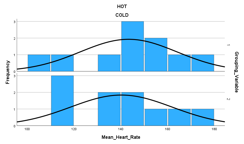
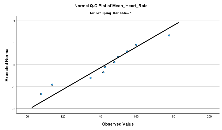
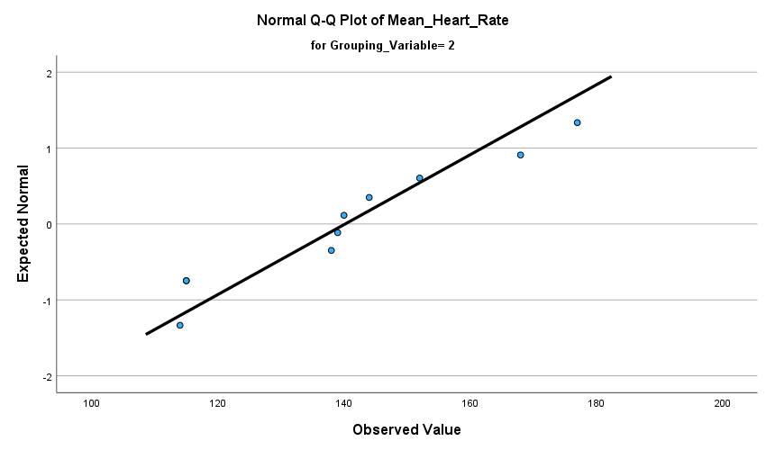
1. Was the assumption of normality met and how do you know?

The assumption of normality was met because Sig. for Mean Heart Rate value 1=.739 and Sig. for Mean Heart Rate value 2=.311. They were both larger than .05.

Table 2. PASTE Tests of NORMALITY table BELOW

Tests of Normality
	Grouping_Variable	Kolmogorov-Smirnova	Shapiro-Wilk
	Statistic	df	Sig.	Statistic	df	Sig.
Mean_Heart_Rate	1	.175	10	.200*	.956	10	.739
2	.177	10	.200*	.914	10	.311
*. This is a lower bound of the true significance.
a. Lilliefors Significance Correction

Figure 1. PASTE Histogram with normal curve for each variable BELOW

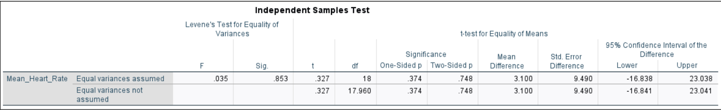
\fNormal Q-Q Plot of Mean_Heart Rate for Grouping_Variable= 1 2 O O Expected Normal 0 -1 -2 100 120 140 160 180 200 Observed ValueNormal Q-Q Plot of Mean_Heart Rate for Grouping_Variable= 2 2 O O O Expected Normal 0 -1 -2 100 120 140 160 180 200 Observed Value\fIndependent Samples Test Levene's Test for Equality of Variances t-test for Equality of Means 95% Confidence Interval of the Significance Mean Std. Error Difference F Sig df One-Sided p Two-Sided p Difference Difference Lower Upper Mean_Heart_Rate Equal variances assumed 035 853 .327 18 374 748 3.100 9.490 -16.838 23.038 Equal variances not .327 17.960 .374 748 3.100 9.490 -16.841 23.041 assumed