Please Help me Solve this.

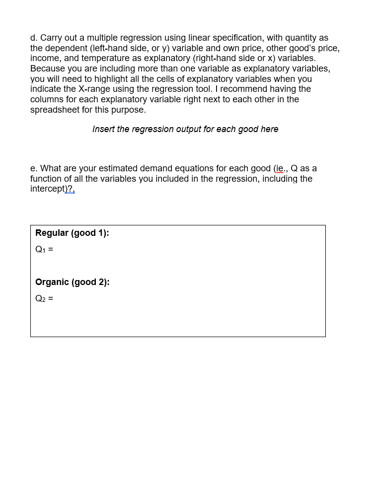
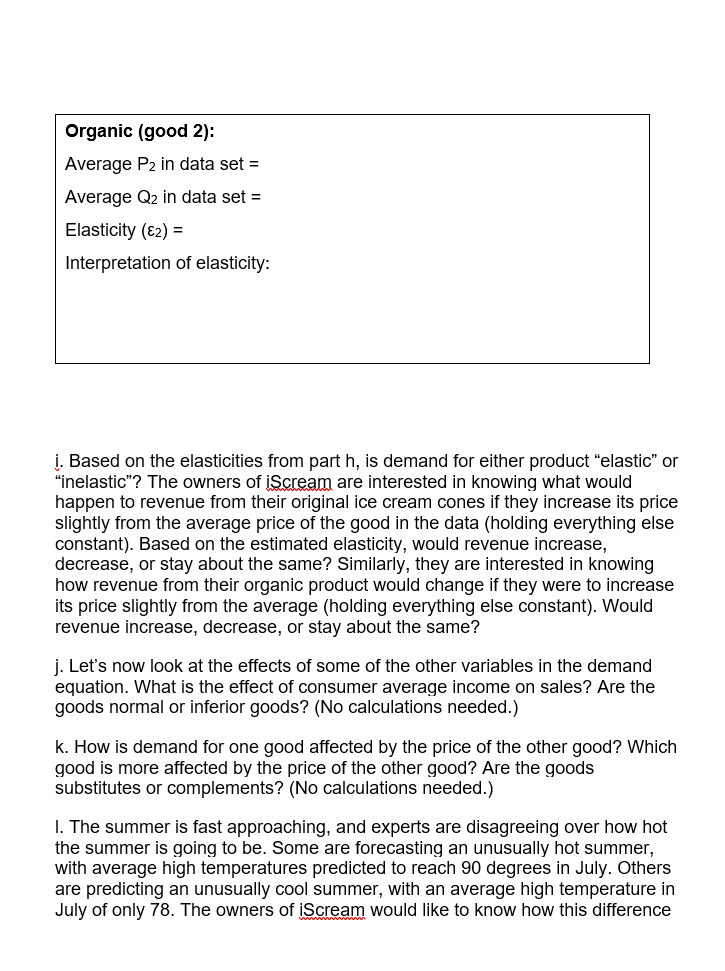
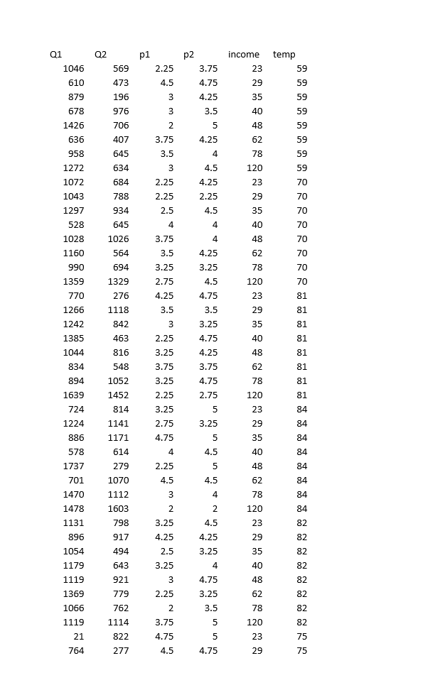
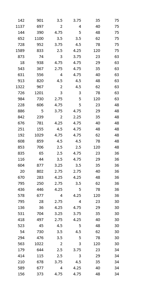
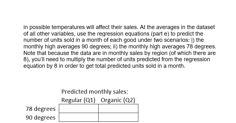
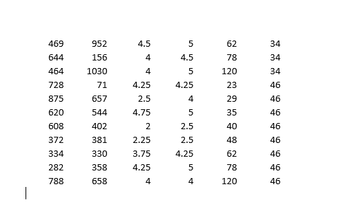
Demand Estimation Assignment iScream Ice lCream Co. iScream is a Chicago start-up that sells ice cream in several mobile ice cream trucks. The main innovative feature of their business is the implementation of a smart phone app that allows customers to locate trucks and request service. iScream has been in business for a little over a year, and offers just two products: regular vanilla ice cream cones and organic, low-fat ice cream cones {each with several toppings that are available at no extra cost}. Based on your previous recommendation, the rm has frequently (for a month at a time} experimented with changing the prices of each of their products in eight equally-populated regions of the city throughout the rst year, and has kept monthly data on their sales and prices of both products. They would now like you to help them gain some insights from the data. While you know relatively little about the ice cream business, you are well aware that factors other than prices are likely to affect demand for a product. Because, through the app, they have information on time and location of sale, you are able to get data on the average household income (in thousands of $1 in the region of sale, as well as the average daily high temperature during the month of sale. The available data can be found in the excel le, \"iScream_data.xlsx". Your goal is to carry out a multiple regression analysis of the data {using Excel}, with particular focus on estimating the price elasticities of demand for both the rm's products. You will be led through this analysis below. Please carry out the following steps and answer the associated questions. Please clearly answer each question below, with the answers or relevant Excel output, like graphs and regression output, inserted into this document (you can copy and paste from Excel}. 1} Begin by looking at the relationship between each product and its own price. For both products separately, dolanswer the following: a. First create a scatter plot of price {on the vertical axis} and quantity sold {on the horizontal axis}. Insert a trend line into each graph and display the equation of the line. This is a crude measure of the inverse demand curve. From the equation of the trendline, ll in the equation of the inverse demand curve for each good in the box below. insert separate graphs for each good here Regular [good 1 l: Inverse demand equation: P1 2 Organic [good 2!: Inverse demand equation: P2 = o. Is there a negative relationship between quantity sold and the product's price? Provide an economic [or managerial} interpretation of the slope of these lines. tie, what do these specic numbers mean?) We are now interested in estimating the demand function, with Quantity {Q} as the dependent variable and price {P} as the explanatory variable {as opposed to the inverse demand function, with P as the dependent variable and Q as the explanatory variable, graphed above}. We know that demand for a product is not onlv inuenced bv its price, but also the price of the other product, among other variables. So instead ofjust graphing the relationship between G and P, similar to what we did above, we will use Excel's Regression tool, as this will allow us to control for other variables. {See section 3.2 in the textbook for an example of using this tool to estimate a simple inverse demand curve. See also the example \"Example Demand Estimation" le in folder Unit 1F). We will use the results from the regressions to answer several questions. For each good, dotanswer the following {d-l): d. Carry out a multiple regression using linear specication, with quantity as the dependent {left-hand side, or y} variable and own price, other goods price, income, and temperature as explanatory {right-hand side or x) variables. Because you are including more than one variable as explanatory variables, you will need to highlight all the cells of explanatory variables when you indicate the Xrange using the regression tool. | recommend having the columns for each explanatory variable right next to each other in the spreadsheet for this purpose. Insert the regression output for each good here e. What are your estimated demand equations for each good (jg, Q as a function of all the variables you included in the regression, including the intercept; Regular [good 1]: Organic [good 2]: CI: = f. What are the Rsquared statistics from each regression? For which product does the demand function explain more of the variation in sales? g. Let's now focus on the effect of a good's own price. What is the coefcient estimate for that same good's price? Provide an economic interpretation of those numbers (egg, by how much does quantity vary with a change in price)? Given the standard errors or the p-values given in the regressions, are these coefcient estimates statistically signicant at the 5% signicance level? h. We are interested in how responsive consumers are to changes in price for each good. To quantify their responsiveness, calculate the pnice elasticity of demand for each product using the regression estimates from part d (see equation 3.6 or refer to GSA 3.2 in the textbook}. As you know, elasticity will vary along the linear demand curve, so you'll need to pick a point at which to calculate the elasticities. Choose the product's average Q and average P in the dataset. Interpret these elasticities (jg, quantitatively, what do these particular numbers mean?}. ls demand for either product elastic or inelastic? Regular [good 1]: Average P1 in data set = Average C11 in data set = Elasticity {E1} = Interpretation of elasticity: Organic [good 2]: Average P2 in data set = Average Q: in data set = Elasticity (2) = Interpretation of elasticity: 1. Based on the elasticities from part h, is demand for either product \"elastic" or \"inelastic"? The owners of igrgml are interested in knowing what would happen to revenue from their original ice cream cones if they increase its price slightly from the average price of the good in the data (holding everything else constant}. Based on the estimated elasticity, would revenue increase, decrease, or stay about the same? Similarly, they are interested in knowing how revenue from their organic product would change if they were to increase its price slightly from the average {holding everything else constant}. Would revenue increase, decrease, or stay about the same? j. Let's now look at the effects of some of the other variables in the demand equation. What is the effect of consumer average income on sales? Are the goods normal or interior goods? (No calculations needed.) k. How is demand for one good affected by the price of the other good? Which good is more affected by the price of the other good? Are the goods substitutes or complements? {No calculations needed.) |. The summer is fast approaching, and experts are disagreeing over how hot the summer is going to be. Some are forecasting an unusually hot summer, with average high temperatures predicted to reach 90 degrees in July. Others are predicting an unusually cool summer, with an average high temperature in July of only T3. The owners of iScream would like to know how this difference in possible temperatures will affect their sales. At the averages in the dataset of all other variables, use the regression equations {part e} to predict the number of units sold in a month of each good under two scenarios: 1} the monthly,r high averages 9-D degrees; ii} the monthlv high averages T8 degrees. Note that because the data are in monthlyr sales by region {of which there are 8}, you'll need to multiply:r the number of units predicted from the regression equation by B in order to get total predicted units sold in a month. Predicted monthlvr sales: Regular {[11} Organic {[12} Y8 degrees 9D degrees Q1 Q2 p1 p2 income temp 1046 569 2.25 3.75 23 59 610 473 4.5 4.75 29 59 879 196 3 4.25 35 59 678 976 3 3.5 40 59 1426 706 5 48 59 636 107 3.75 4.25 62 59 958 645 3.5 4 78 59 1272 634 3 4.5 120 59 1072 684 2.25 4.25 23 70 1043 788 2.25 2.25 29 70 1297 934 2.5 4.5 35 70 528 645 4 4 40 70 1028 1026 3.75 4 48 70 1160 564 3.5 4.25 62 70 990 694 3.25 3.25 78 70 1359 1329 2.75 4.5 120 70 770 276 4.25 4.75 23 81 1266 1118 3.5 3.5 29 81 1242 842 3 3.25 35 81 1385 463 2.25 4.75 40 81 1044 816 3.25 4.25 48 81 834 548 3.75 3.75 62 81 894 1052 3.25 4.75 78 81 1639 1452 2.25 2.75 120 81 724 814 3.25 5 23 84 1224 1141 2.75 3.25 29 84 886 1171 4.75 5 35 84 578 614 4 4.5 40 84 1737 279 2.25 5 48 84 701 1070 4.5 4.5 62 84 1470 1112 3 4 78 84 1478 1603 2 2 120 84 1131 798 3.25 4.5 23 82 896 917 4.25 4.25 29 82 1054 494 2.5 3.25 35 82 1179 643 3.25 4 40 82 1119 921 3 4.75 48 82 1369 779 2.25 3.25 62 82 1066 762 2 3.5 78 82 1119 1114 3.75 5 120 82 21 822 4.75 5 23 75 764 277 4.5 4.75 29 75\f469 952 4.5 5 62 34 644 156 4 4.5 78 34 464 1030 4 5 120 34 728 71 4.25 4.25 23 46 875 657 2.5 4 29 46 620 544 4.75 5 35 46 608 402 2 2.5 40 46 372 381 2.25 2.5 48 46 334 330 3.75 4.25 62 46 282 358 4.25 5 78 46 788 658 4 4 120 46