Please help me this problem. I have started it but I have no idea how to find Min and Max expected returns, standard deviation and other metrics that need to be solved for this problem.

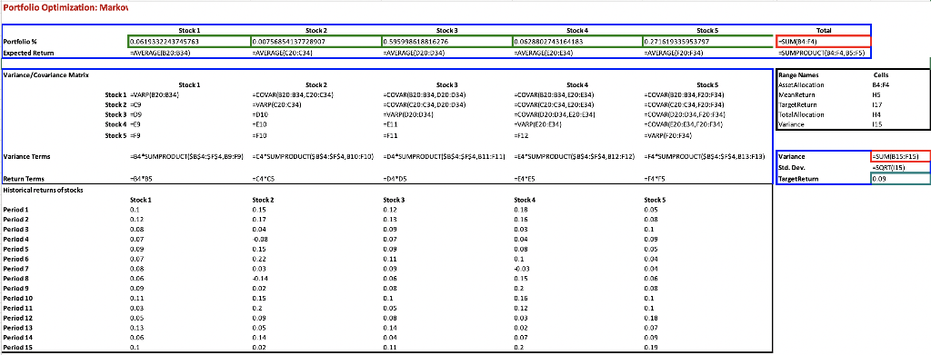
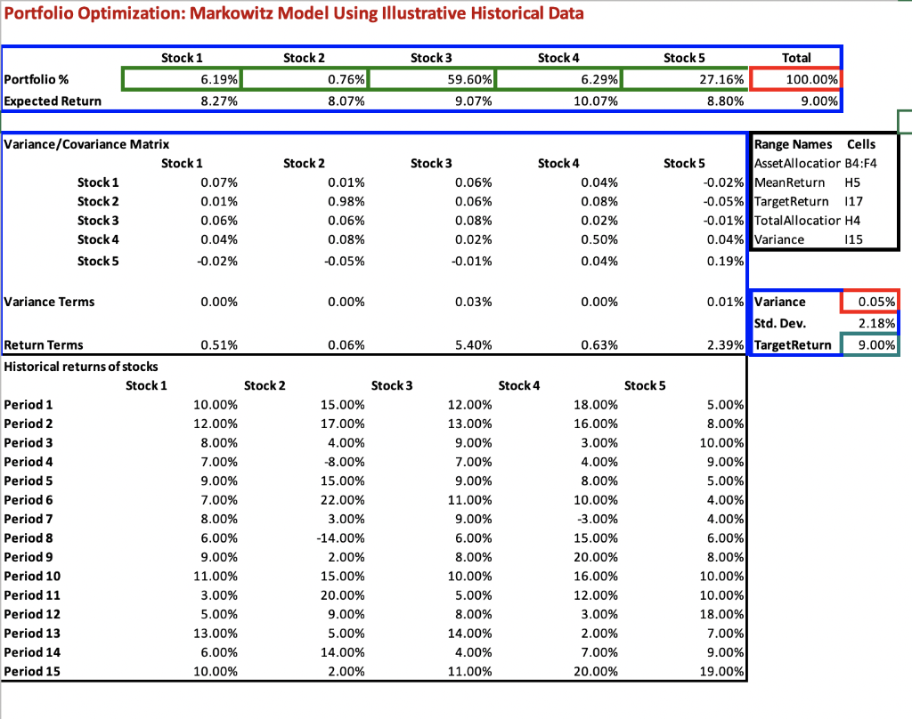
2.2 (30 points) The efficient frontier is defined by the entire set of optimal portfolios that offer the highest expected return for stated (fixed) levels of risk, or - alternatively - offer the lowest risk for a given level of expected return. In our Markowitz model formulation, we followed the second approach. Suboptimal portfolios do not provide enough (estimated) return for the given level of risk, or have higher than necessary risk for a given level of expected return. Consequently, we are interested in finding (estimating) optimal portfolios which are represented by points on the efficient frontier. Risk can be modeled e.g., by portfolio variance, or (equivalently) by the standard deviation of the portfolio. Based on your revised data set (using all 15 data for each stock), find the minimal and maximal expected return that can be achieved. You can round your expected return data: e.g., 6.86% can be rounded up to 7% and 20.2% can be rounded down to 20%. Divide the range between these minimal and maximal expected return data into steps of 0.5%: these will be your target return parameters. In the above example, you will consider the values t = 7%, 7.5%, 8%, ..., 19%, 19.5%, 20%. Solve the resulting portfolio optimization problems, by minimizing the standard deviation of the portfolio. Based on your results, create a graph that summarizes these results. This graph estimates points on the efficient frontier based on your data set. Draw your conclusion regarding the tradeoff between portfolio return and risk in one or two sentences. Portfolio Optimization: Marko Portfolio % Expected Retur Variance/Covariance Matrix Variance Terms Return Terms Historical returns of stocks Period 1 Period 2 Period 3 Period 4 Period 5 Period 6 Period 7 Period 8 Period 9 Perlod 10 Period 11 Period 12 Period 13 Period 14 Period 15 Stock 5 Total Stock 1 0.0619332243745763 AVERAGE(B20:834) Stock 2 0.00756854137728907 AVERAGE/C20:34) Stock 3 0.595998618816276 AVERAGE(D20:034) Stock 4 0.0628802743164183 AVERAGE(E20:E34) -SUM/B4 F41 0.271619335953797 AVERAGE/F20:F34) SUMPRODUCT(84:F4,95:F5) Stock 1 VARP(820:834) Stock 2 =CCVAR(320 834,C20:34) =VARP(C20 C34) Stock 1 Stock 2 =C9 Stock 3 -09 Stock49 Stock 5 =9 Stock 3 -COVAR(B20:834,D20:034) =COVAR(C20:C34,D20 D34) =VARPID20:034) -E11 =F11 Stock 4 -COVAR(B20:834, E20:E34) -COVARIC20:C34, E20:E34) -COVARID20:034,E20:34) -VARPIE20 E341 =F12 Range Names AssetAllocation. MeanReturn Target Return TotalAllocation Variance Stock 5 -CCVAR(320:834,F20:F34) =COVAR(C20 C34,F20:F34) -COVAR(020:034,F20 F34) -COVAR(E20:E34,F20:F34) =VARP(-20:F34) =D10 -E10 =F10 -84*SUMPRODUCT($B$4:$F$4,89:F9 =C4 SUMPRODUCT($B$4:$F$4,810:F10) =D4 SUMPRODUCT($B$4:$F$4,811:F11) =E4"SUMPRODUCT($B$4:$F$4,812:F12) F4*SUMPRODUCT($B$4:$F$4,813:F13) Variance Std. Dev. -64*85 -C4 C5 -D4 D5 -E4-E5 -F4F5 TargetRetum Stock: Stock 2 0.15 Stock 3 0.12 Stock 4 0.18 Stock 5 0.05 0.1 0.12 0.17 0.13 0.16 0.08 0.08 0.04 0.09 0.03 0.1 0.07 -0.08 0.07 0.04 0.09 0.09 0.15 0.09 0.09 0.05 0.07 0.22 0.11 0.1 0.04 0.08 0.03 0.09 0:03 0.04 0.06 -0.14 0.06 0.15 0.06 0.09 0.02 0.08 0.2 0.08 0.11 0.15 0.1 0.16 0.1 0.03 0.2 0.05 0.12 0.1 0.05 0.09 0.08 0.03 0.18 0.13 0.05 0.14 0.02 0.07 0.06 0.14 0.04 0.07 0.09 0.1 0.02 0.11 0.2 0.19 Cells B4:F4 HS H4 115 =SUMIB15:F15) -SORT(115) 0.09 Portfolio Optimization: Markowitz Model Using Illustrative Historical Data Stock 1 Stock 2 Stock 3 Stock 4 6.19% Portfolio % Expected Return 0.76% 8.07% 59.60% 9.07% 8.27% Variance/Covariance Matrix Stock 1 0.07% 0.01% 0.06% Stock 2 0.01% 0.98% 0.06% Stock 3 0.06% 0.06% 0.08% Stock 4 0.04% 0.08% 0.02% Stock 5 -0.02% -0.05% -0.01% Variance Terms 0.00% 0.00% 0.03% Return Terms 0.51% 0.06% 5.40% Historical returns of stocks Stock 1 Period 1 10.00% 15.00% 12.00% Period 2 12.00% 17.00% 13.00% Period 3 8.00% 4.00% 9.00% Period 4 7.00% -8.00% 7.00% Period 5 9.00% 15.00% 9.00% Period 6 7.00% 22.00% 11.00% Period 7 8.00% 3.00% 9.00% Period 8 6.00% -14.00% 6.00% Period 9 9.00% 2.00% 8.00% Period 10 11.00% 15.00% 10.00% Period 11 3.00% 20.00% 5.00% Period 12 5.00% 9.00% 8.00% Period 13 13.00% 5.00% 14.00% Period 14 6.00% 14.00% 4.00% Period 15 10.00% 2.00% 11.00% Stock 1 Stock 2 Stock 2 Stock 3 Stock 3 6.29% 10.07% 0.04% 0.08% 0.02% 0.50% 0.04% 0.00% 0.63% 18.00% 16.00% 3.00% 4.00% 8.00% 10.00% -3.00% 15.00% 20.00% 16.00% 12.00% 3.00% 2.00% 7.00% 20.00% Stock 4 Stock 4 Stock 5 27.16% 8.80% Stock 5 100.00% 9.00% Range Names Cells Asset Allocatior B4:F4 -0.02% Mean Return H5 -0.05% Target Return 117 -0.01% Total Allocatior H4 0.04% Variance 115 0.19% 0.01% Variance Std. Dev. 2.39% TargetReturn 5.00% 8.00% 10.00% 9.00% 5.00% 4.00% 4.00% 6.00% 8.00% 10.00% 10.00% 18.00% 7.00% 9.00% 19.00% Stock 5 Total 0.05% 2.18% 9.00% Solver Parameters Value Of: Set Objective: Variance To: Max Min By Changing Variable Cells: AssetAllocation Subject to the Constraints: Add MeanReturn >= TargetReturn TotalAllocation = 1 Change Delete Reset All Load/Save Make Unconstrained Variables Non-Negative Select a Solving Method: GRG Nonlinear Options Solving Method Select the GRG Nonlinear engine for Solver Problems that are smooth nonlinear. Select the LP Simplex engine for linear Solver Problems, and select the Evolutionary engine for Solver problems that are non- smooth. Close Solve 0 E F 1 C . C 2.2 (30 points) The efficient frontier is defined by the entire set of optimal portfolios that offer the highest expected return for stated (fixed) levels of risk, or - alternatively - offer the lowest risk for a given level of expected return. In our Markowitz model formulation, we followed the second approach. Suboptimal portfolios do not provide enough (estimated) return for the given level of risk, or have higher than necessary risk for a given level of expected return. Consequently, we are interested in finding (estimating) optimal portfolios which are represented by points on the efficient frontier. Risk can be modeled e.g., by portfolio variance, or (equivalently) by the standard deviation of the portfolio. Based on your revised data set (using all 15 data for each stock), find the minimal and maximal expected return that can be achieved. You can round your expected return data: e.g., 6.86% can be rounded up to 7% and 20.2% can be rounded down to 20%. Divide the range between these minimal and maximal expected return data into steps of 0.5%: these will be your target return parameters. In the above example, you will consider the values t = 7%, 7.5%, 8%, ..., 19%, 19.5%, 20%. Solve the resulting portfolio optimization problems, by minimizing the standard deviation of the portfolio. Based on your results, create a graph that summarizes these results. This graph estimates points on the efficient frontier based on your data set. Draw your conclusion regarding the tradeoff between portfolio return and risk in one or two sentences. Portfolio Optimization: Marko Portfolio % Expected Retur Variance/Covariance Matrix Variance Terms Return Terms Historical returns of stocks Period 1 Period 2 Period 3 Period 4 Period 5 Period 6 Period 7 Period 8 Period 9 Perlod 10 Period 11 Period 12 Period 13 Period 14 Period 15 Stock 5 Total Stock 1 0.0619332243745763 AVERAGE(B20:834) Stock 2 0.00756854137728907 AVERAGE/C20:34) Stock 3 0.595998618816276 AVERAGE(D20:034) Stock 4 0.0628802743164183 AVERAGE(E20:E34) -SUM/B4 F41 0.271619335953797 AVERAGE/F20:F34) SUMPRODUCT(84:F4,95:F5) Stock 1 VARP(820:834) Stock 2 =CCVAR(320 834,C20:34) =VARP(C20 C34) Stock 1 Stock 2 =C9 Stock 3 -09 Stock49 Stock 5 =9 Stock 3 -COVAR(B20:834,D20:034) =COVAR(C20:C34,D20 D34) =VARPID20:034) -E11 =F11 Stock 4 -COVAR(B20:834, E20:E34) -COVARIC20:C34, E20:E34) -COVARID20:034,E20:34) -VARPIE20 E341 =F12 Range Names AssetAllocation. MeanReturn Target Return TotalAllocation Variance Stock 5 -CCVAR(320:834,F20:F34) =COVAR(C20 C34,F20:F34) -COVAR(020:034,F20 F34) -COVAR(E20:E34,F20:F34) =VARP(-20:F34) =D10 -E10 =F10 -84*SUMPRODUCT($B$4:$F$4,89:F9 =C4 SUMPRODUCT($B$4:$F$4,810:F10) =D4 SUMPRODUCT($B$4:$F$4,811:F11) =E4"SUMPRODUCT($B$4:$F$4,812:F12) F4*SUMPRODUCT($B$4:$F$4,813:F13) Variance Std. Dev. -64*85 -C4 C5 -D4 D5 -E4-E5 -F4F5 TargetRetum Stock: Stock 2 0.15 Stock 3 0.12 Stock 4 0.18 Stock 5 0.05 0.1 0.12 0.17 0.13 0.16 0.08 0.08 0.04 0.09 0.03 0.1 0.07 -0.08 0.07 0.04 0.09 0.09 0.15 0.09 0.09 0.05 0.07 0.22 0.11 0.1 0.04 0.08 0.03 0.09 0:03 0.04 0.06 -0.14 0.06 0.15 0.06 0.09 0.02 0.08 0.2 0.08 0.11 0.15 0.1 0.16 0.1 0.03 0.2 0.05 0.12 0.1 0.05 0.09 0.08 0.03 0.18 0.13 0.05 0.14 0.02 0.07 0.06 0.14 0.04 0.07 0.09 0.1 0.02 0.11 0.2 0.19 Cells B4:F4 HS H4 115 =SUMIB15:F15) -SORT(115) 0.09 Portfolio Optimization: Markowitz Model Using Illustrative Historical Data Stock 1 Stock 2 Stock 3 Stock 4 6.19% Portfolio % Expected Return 0.76% 8.07% 59.60% 9.07% 8.27% Variance/Covariance Matrix Stock 1 0.07% 0.01% 0.06% Stock 2 0.01% 0.98% 0.06% Stock 3 0.06% 0.06% 0.08% Stock 4 0.04% 0.08% 0.02% Stock 5 -0.02% -0.05% -0.01% Variance Terms 0.00% 0.00% 0.03% Return Terms 0.51% 0.06% 5.40% Historical returns of stocks Stock 1 Period 1 10.00% 15.00% 12.00% Period 2 12.00% 17.00% 13.00% Period 3 8.00% 4.00% 9.00% Period 4 7.00% -8.00% 7.00% Period 5 9.00% 15.00% 9.00% Period 6 7.00% 22.00% 11.00% Period 7 8.00% 3.00% 9.00% Period 8 6.00% -14.00% 6.00% Period 9 9.00% 2.00% 8.00% Period 10 11.00% 15.00% 10.00% Period 11 3.00% 20.00% 5.00% Period 12 5.00% 9.00% 8.00% Period 13 13.00% 5.00% 14.00% Period 14 6.00% 14.00% 4.00% Period 15 10.00% 2.00% 11.00% Stock 1 Stock 2 Stock 2 Stock 3 Stock 3 6.29% 10.07% 0.04% 0.08% 0.02% 0.50% 0.04% 0.00% 0.63% 18.00% 16.00% 3.00% 4.00% 8.00% 10.00% -3.00% 15.00% 20.00% 16.00% 12.00% 3.00% 2.00% 7.00% 20.00% Stock 4 Stock 4 Stock 5 27.16% 8.80% Stock 5 100.00% 9.00% Range Names Cells Asset Allocatior B4:F4 -0.02% Mean Return H5 -0.05% Target Return 117 -0.01% Total Allocatior H4 0.04% Variance 115 0.19% 0.01% Variance Std. Dev. 2.39% TargetReturn 5.00% 8.00% 10.00% 9.00% 5.00% 4.00% 4.00% 6.00% 8.00% 10.00% 10.00% 18.00% 7.00% 9.00% 19.00% Stock 5 Total 0.05% 2.18% 9.00% Solver Parameters Value Of: Set Objective: Variance To: Max Min By Changing Variable Cells: AssetAllocation Subject to the Constraints: Add MeanReturn >= TargetReturn TotalAllocation = 1 Change Delete Reset All Load/Save Make Unconstrained Variables Non-Negative Select a Solving Method: GRG Nonlinear Options Solving Method Select the GRG Nonlinear engine for Solver Problems that are smooth nonlinear. Select the LP Simplex engine for linear Solver Problems, and select the Evolutionary engine for Solver problems that are non- smooth. Close Solve 0 E F 1 C . C