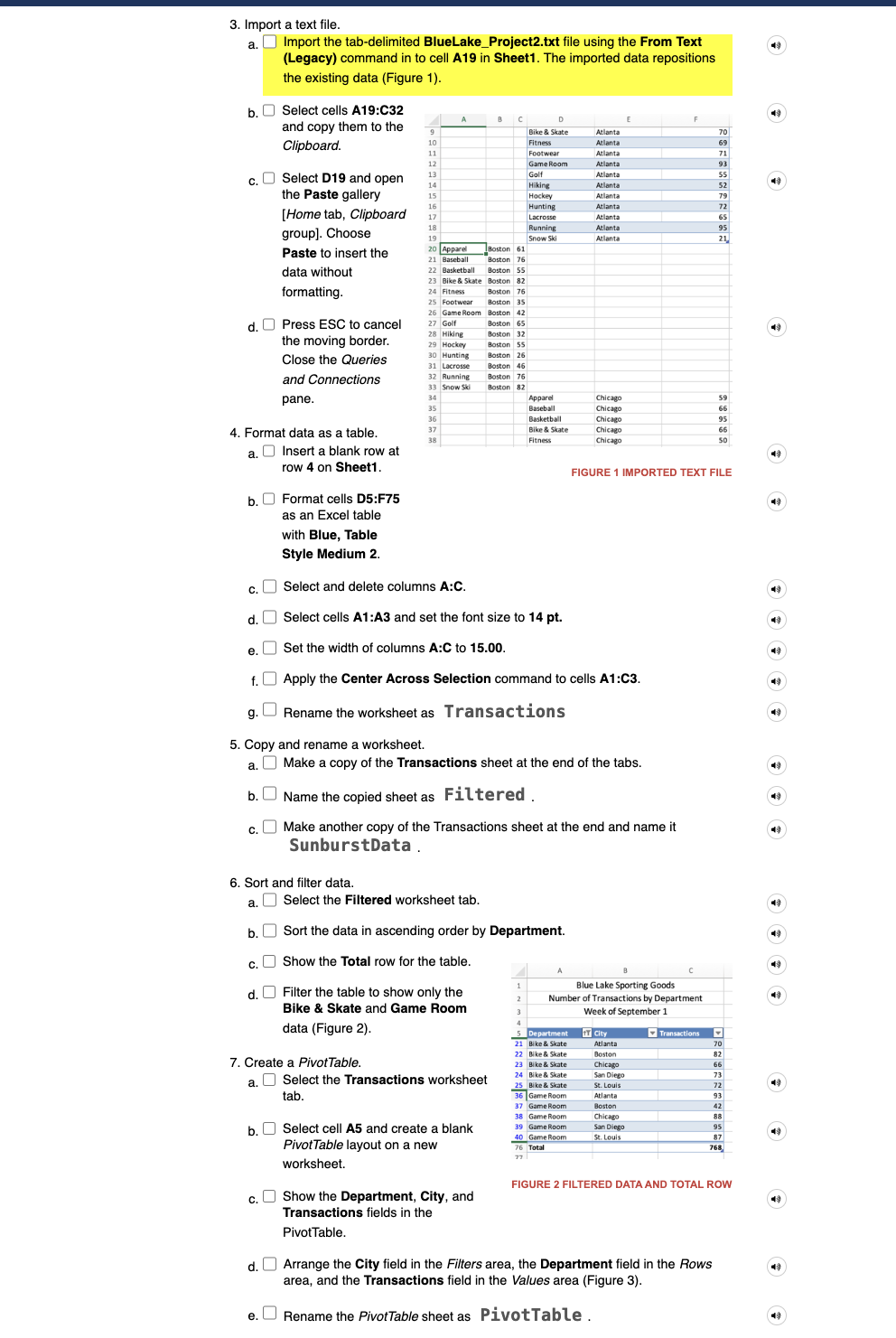
Question: PLease help me with doing this, I am struggling and need help with completing this h . Return to the SunburstChart sheet. When values are
PLease help me with doing this, I am struggling and need help with completing this
h Return to the SunburstChart sheet. When values are too small to scale, the
slice displays as blank Figure
FIGURE SUNBURST CHART
Name a cell range and insert a column.
a Select the LookupData tab name.
b Select cells A:A and name the range Cities.
c Select cells B:B and name the range TaxRates.
d Select the TransactionData sheet and insert a column at column C
e Select cell C and type Tax Rate
Build a XLOOKUP formula.
a Select cell C on the TransactionData tab.
FIGURE XLOOKUP ARGUMENTS
b Build a XLOOKUP formula to lookup the value in cell A in the Cities range
and display the tax rate. Figure
c Copy the XLOOKUP formula in column C and format the results as Percent
Style with decimals.
Use order of precedence in a formula.
a Select cell D on the TransactionData tab.
b quad Type to start a formula and click cell B
c Type to multiply and enter the opening parenthesis.
d Type and click cell C The sales amount is multiplied by plus the tax
rate to calculate the total bill.
e Press Enter. The missing parenthesis is noted.
f Click Yes to accept the correction.
Create and format a Clustered Column PivotChart.
a Select cell A in the PivotTable and insert a Clustered Column PivotChart.
b Position and size the chart object to start at cell D and reach to cell M
c Select one of the columns in the PivotChart and click the Format Pane button
PivotChart Format tab, Format group
d Find and expand the Fill command group and select the Vary colors by
point box.
e Close the Format Data Series task pane.
f Click the Total title box in the chart and edit the text to display # of
Transactions by Department.
g Apply a Black, Text outline with a weight of pt to the chart object.
h Hide the display of Field Buttons in the PivotChart. Note: Mac users please
skip this step and proceed to the next step.
i Select cell AFigure
Create and format a sunburst chart.
a Select the SunburstData tab name.
b Select column B cut it and insert it at column A to rearrange the data so that
the City column is column A The top level in a hierarchy chart should be
leftmost in the data.
c Select cells B:B and move them to column A
d Select cells A:C and apply the Center Across Selection command.
e Select cell A and insert a Sunburst chart on its own sheet named
SunburstChart.
f Edit the Chart Title placeholder text to display # of Transactions
by City and Department. The city names are the inner ring of
the chart, the top level in the hierarchy.
g Return to the SunburstData sheet and filter the table to show all departments
except Apparel, Footwear, and Running.
Finalize the workbook by setting page
options and document properties.
a Open the Properties dialog box
File menu
b Select the Summary tab.
c Type Transactions
Data in the Title box; type
your name in the Author box.
d Click the Comments box, type First week of September,
and return to the workbook Figure
e Select the PivotTable sheet tab. Change the page orientation to landscape
and scale the sheet to fit a single page.
f Select the Transactions sheet tab and scale it to fit a single page.
Save and close the workbook Figure
Upload and save your project file.
Submit project for grading.

Step by Step Solution
There are 3 Steps involved in it
1 Expert Approved Answer
Step: 1 Unlock


Question Has Been Solved by an Expert!
Get step-by-step solutions from verified subject matter experts
Step: 2 Unlock
Step: 3 Unlock


