please help me with the formula

To find the Final mark

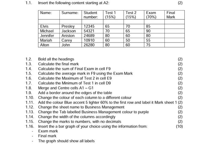
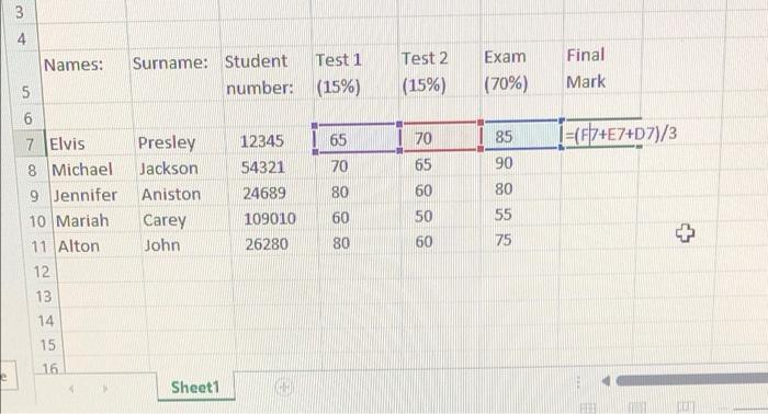
1.1. Insert the following content starting at A2: (2) Name: Surname: Student number: Test 1 (15%) Test 2 (15%) Exam (70%) Final Mark Elvis Michael Jennifer Mariah Alton Presley Jackson Aniston Carey John 12345 54321 24689 10910 26280 65 70 80 60 80 70 65 60 50 60 85 90 80 55 75 1.2. Bold all the headings 1.3. Calculate the final mark 1.4. Calculate the sum of Final Exam in cell F9 1.5. Calculate the average mark in F9 using the Exam Mark 1.6. Calculate the Maximum of Test 2 in cell E9 1.7. Calculate the Minimum of Test 1 in cell D9 1.8. Merge and Centre cells A1 - G1 1.9. Add a border around the edges of the table 1.10. Change the colour of each column to a different colour 1.11. Add the colour Blue accent 5 lighter 60% to the first row and label it Mark sheet 1 (2) 1.12. Change the sheet name to Business Management 1.13. Change the Tab labelled Business Management colour to purple (2) 1.14. Change the width of the columns accordingly 1.15. Change the marks to numbers, with no decimals 1.16. Insert the a bar graph of your choice using the information from: (10) Exam mark Final mark The graph should show all labels ODBROOOOOOOOOO 3 4 Names: Surname: Student Test 1 number: (15%) Test 2 (15%) Exam (70%) Final Mark 5 6 70 I=(F7+E7+D7)/3 Presley Jackson Aniston Carey John 12345 54321 24689 109010 26280 65 70 80 7 Elvis 8 Michael 9 Jennifer 10 Mariah 11 Alton 12 13 14 15 65 60 50 60 85 90 80 55 75 60 + 80 16 Sheet1