Please Help!

Perform a PolynomialFeatures transformation, then perform linear regression to calculate the optimal ordinary least squares regression model parameters.

Recreate the first figure by adding the best fit curve to all subplots.

Infer the true model parameters.

a. Perform a polynomial transformation on your features.

b. From the sklearn.linear_model library, import the LinearRegression class. Instantiate an object of this class called model, and fit it to the data. x and y will be your training data and z will be your response. Print the optimal model parameters to the screen by completing the following print() statements.

c. Use the following x_fit and y_fit data to compute z_fit by invoking the model's predict() method. This will allow you to plot the line of best fit that is predicted by the model.

This is the code I need to use to be able to plot the line of best fit.

from mpl_toolkits.mplot3d import Axes3D

fig, axs = plt.subplots(2, 2, figsize=(15, 10), subplot_kw={'projection': '3d'}) axs = axs.ravel()

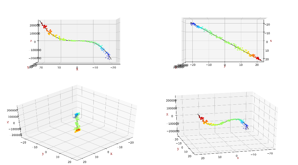
#Image for scatterplot 1 axs[0].scatter3D(x,y,z,c=z, cmap='jet') axs[0].set_xlabel('x', c='r', size =12) axs[0].set_ylabel('y', c='r', size =12) axs[0].set_zlabel('z', c='r', size =12) axs[0].view_init(1,86)

#Image for scatterplot 2 axs[1].scatter3D(x,y,z,c=z, cmap='jet') axs[1].set_xlabel('x', c='r', size =12) axs[1].set_ylabel('y', c='r', size =12) axs[1].set_zlabel('z', c='r', size =12) axs[1].view_init(90,0)

#Image for scatterplot 3 axs[2].scatter3D(x,y,z,c=z, cmap='jet') axs[2].set_xlabel('x', c='r', size =12) axs[2].set_ylabel('y', c='r', size =12) axs[2].set_zlabel('z', c='r', size =12) axs[2].view_init(37,46)

#Image for scatterplot 4 axs[3].scatter3D(x,y,z,c=z, cmap='jet') axs[3].set_xlabel('x', c='r', size =12) axs[3].set_ylabel('y', c='r', size =12) axs[3].set_zlabel('z', c='r', size =12) axs[3].view_init(17,81)

plt.show()

This is what it should look like