please help!

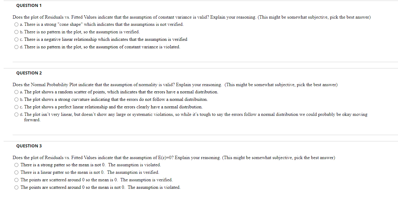
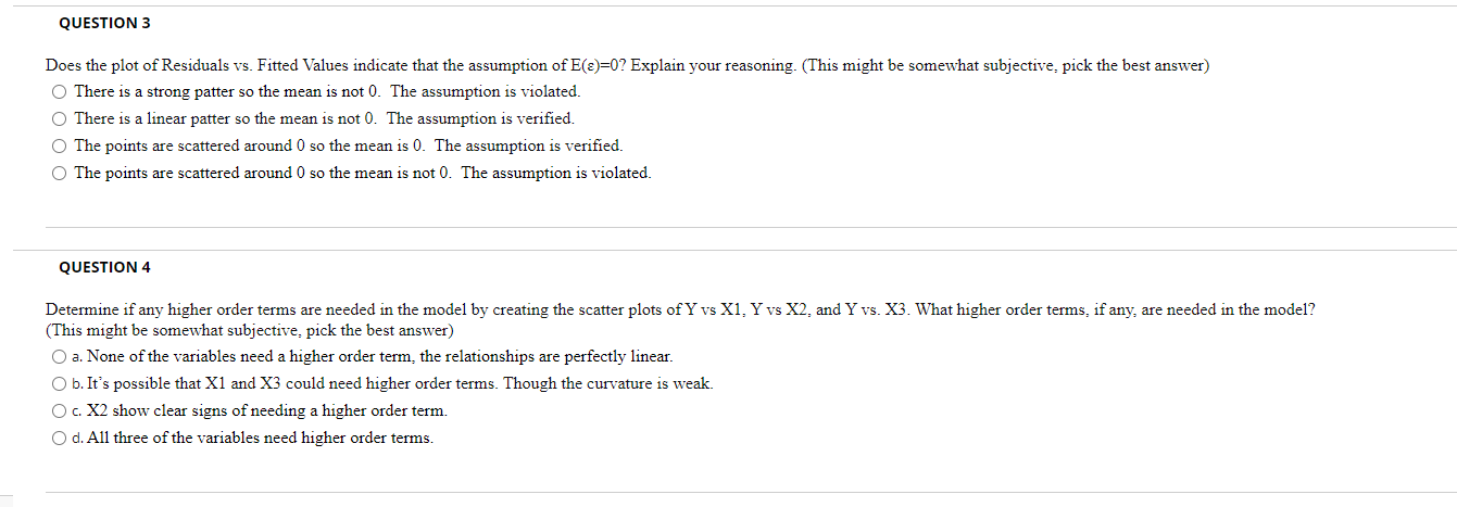
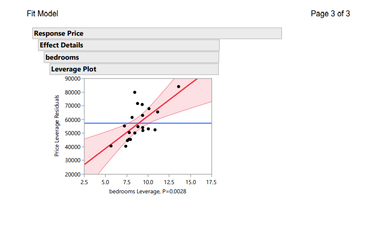
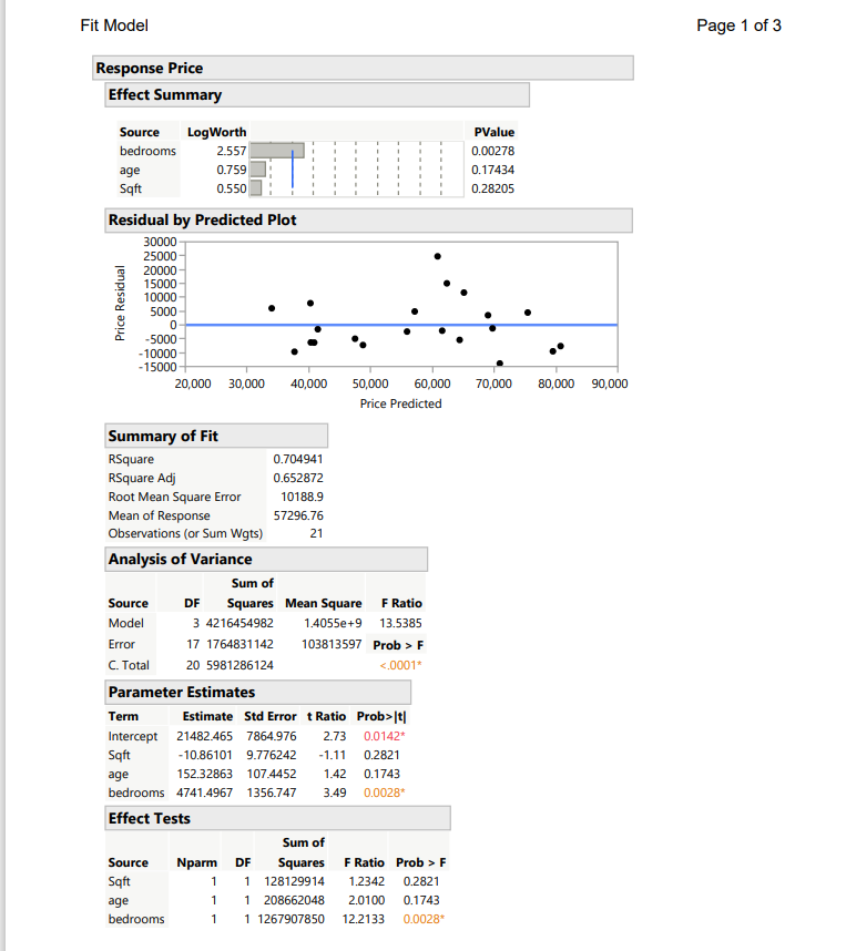
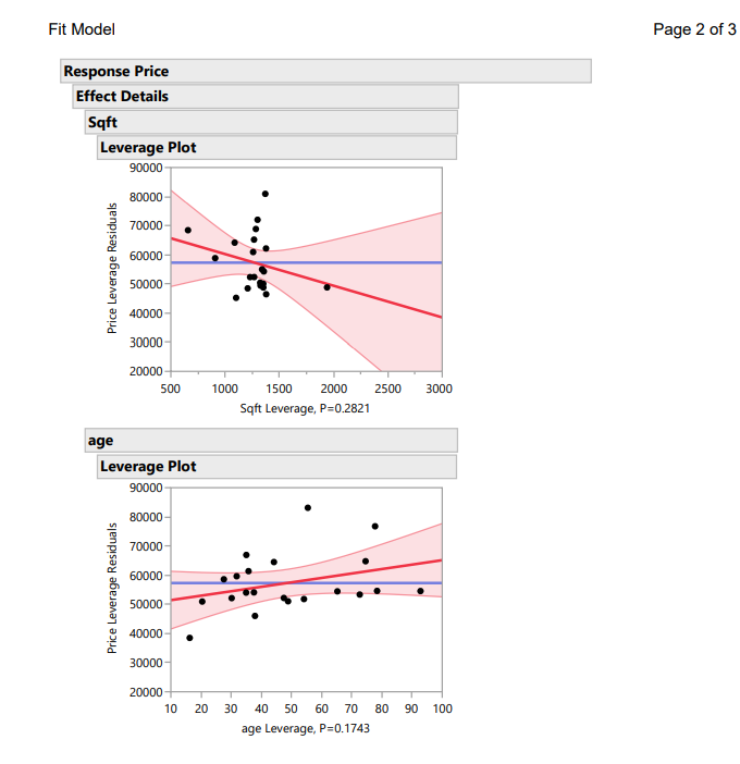
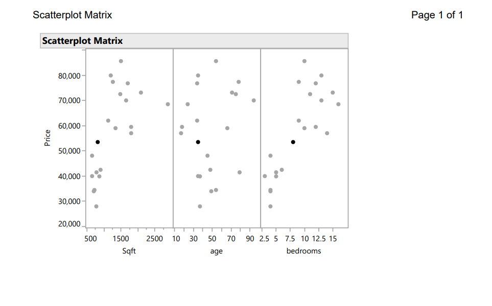
QUESTION 1 Does the plot of Residuals vs. Fitted Values indicate that the assumption of constant variance is valid? Explain your reasoning. (This might be somewhat subjective, pick the best answer) O a. There is a strong "cone shape" which indicates that the assumptions is not verified. O b. There is no pattern in the plot, so the assumption is verified. O c. There is a negative linear relationship which indicates that the assumption is verified O d. There is no pattern in the plot, so the assumption of constant variance is violated. QUESTION 2 Does the Normal Probability Plot indicate that the assumption of normality is valid? Explain your reasoning. (This might be somewhat subjective, pick the best answer) O a. The plot shows a random scatter of points, which indicates that the errors have a normal distribution. O b. The plot shows a strong curvature indicating that the errors do not follow a normal distribuiton. O c. The plot shows a perfect linear relationship and the errors clearly have a normal distribution. O d. The plot isn't very linear, but doesn't show any large or systematic violations, so while it's tough to say the errors follow a normal distribution we could probably be okay moving forward. QUESTION 3 Does the plot of Residuals vs. Fitted Values indicate that the assumption of E(=)=0? Explain your reasoning. (This might be somewhat subjective, pick the best answer) O There is a strong patter so the mean is not 0. The assumption is violated. O There is a linear patter so the mean is not 0. The assumption is verified. O The points are scattered around 0 so the mean is 0. The assumption is verified. O The points are scattered around 0 so the mean is not 0. The assumption is violated.JESTION 3 Does the plot of Residuals vs. Fitted Values indicate that the assumption of E()=0? Explain your reasoning. (This might be somewhat subjective, pick the best answer) O There is a strong patter so the mean is not 0. The assumption is violated. O There is a linear patter so the mean is not 0. The assumption is verified. O The points are scattered around 0 so the mean is 0. The assumption is verified. O The points are scattered around 0 so the mean is not 0. The assumption is violated. QUESTION 4 Determine if any higher order terms are needed in the model by creating the scatter plots of Y vs X1, Y vs X2, and Y vs. X3. What higher order terms, if any, are needed in the model? (This might be somewhat subjective, pick the best answer) O a. None of the variables need a higher order term, the relationships are perfectly linear. O b. It's possible that X1 and X3 could need higher order terms. Though the curvature is weak. O c. X2 show clear signs of needing a higher order term. O d. All three of the variables need higher order terms.Fit Model Page 3 of 3 Response Price Effect Details bedrooms Leverage Plot 90000 80000 70000 60000 Price Leverage Residuals 50000 40000- 30000 20000- 2.5 5.0 7.5 10.0 12.5 15.0 17.5 bedrooms Leverage, P=0.0028Fit Model Page 1 of 3 Response Price Effect Summary Source LogWorth PValue bedrooms 2.557 0.00278 age 0.759 0.17434 Sqft 0.550 0.28205 Residual by Predicted Plot 30000 25000 20000 15000 10000 Price Residual 5000 0- -5000 -10000 -15000 20,000 30,000 40,000 50,000 60,000 70,000 80,000 90,000 Price Predicted Summary of Fit RSquare 0.704941 RSquare Adj 0.652872 Root Mean Square Error 10188.9 Mean of Response 57296.76 Observations (or Sum Wgts) 21 Analysis of Variance Sum of Source DF Squares Mean Square F Ratio Model 3 4216454982 1.4055e+9 13.5385 Error 17 1764831142 103813597 Prob > F C. Total 20 5981286124 <.0001 parameter estimates term estimate std error t ratio prob>|t] Intercept 21482.465 7864.976 2.73 0.0142* Sqft -10.86101 9.776242 -1.11 0.2821 age 152.32863 107.4452 1.42 0.1743 bedrooms 4741.4967 1356.747 0.0028* Effect Tests Sum of Source Nparm DF Squares F Ratio Prob > F Sqft 1 128129914 1.2342 0.2821 age 1 208662048 2.0100 0.1743 bedrooms 1 1267907850 12.2133 0.0028*Fit Model Page 2 of 3 Response Price Effect Details Saft Leverage Plot 90000 80000 70000 60000 Price Leverage Residuals 50000 40000 30000 20000 500 1000 1500 2000 2500 3000 Sqft Leverage, P=0.2821 age Leverage Plot 90000 80000 70000 60000 Price Leverage Residuals 50000 40000 30000 20000- 10 20 30 40 50 60 70 80 90 100 age Leverage, P=0.1743Scatterplot Matrix Page 1 of 1 Scatterplot Matrix 80,000- 70,000 60,000- Price 50,000 40,000- 30,000 20,000 500 1500 2500 10 30 50 70 90 2.5 5 7.5 10 12.5 15 Sqft age bedrooms