please help solve excel below

:

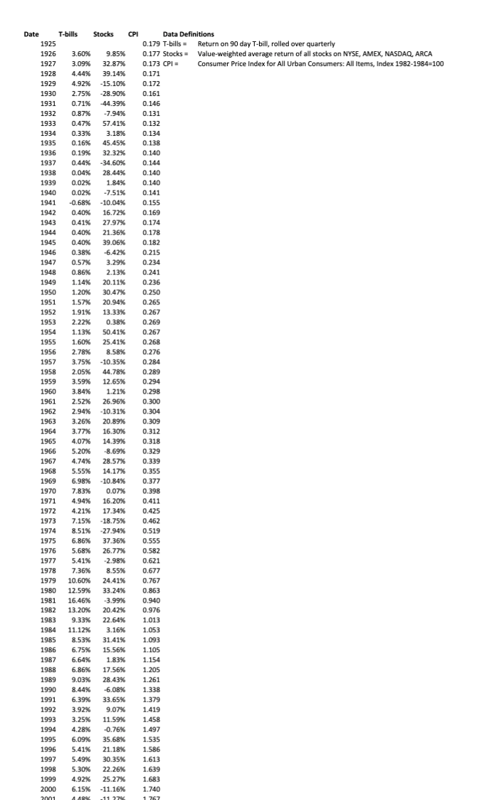
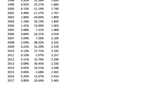
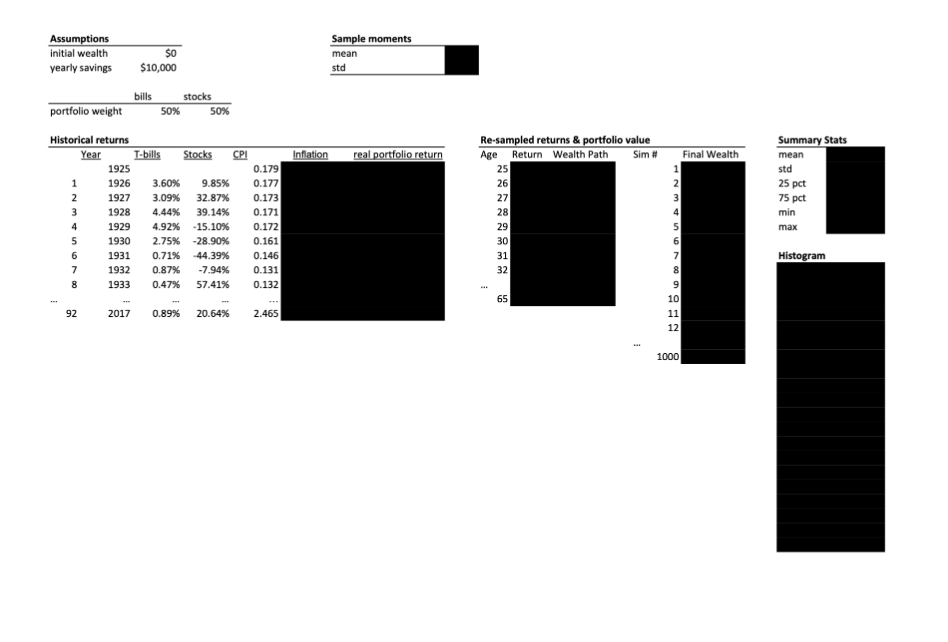
ASSIGNMENT 1 Due: Wednesday, 01.27.21 at 11:59 pm In this assignment, you will use a Monte Carlo simulation to investigate the effect of randomness in returns on an individual's future retirement wealth. Saving for Retirement Assume an investor begins saving for retirement at age 25 and retires at age 65. Each year, she contributes $10, 000 to her retirement account. To keep thing simple, assume that there are 40 annual contributions that occur on the investor's 25-th, 26-th, ...,64-th birthdays, and that the nal retirement wealth is determined on the investor's 65-th birthday.l Savings are invested as follows: 50% in a broad stock market index and 50% in TBills. Your task is to compute the accumulated real retirement savings at age 65 for different return realizations. As explained below, you will generate returns using a Monte Carlo simulation. On Canvas, you can nd an Excel le containing historical net returns on the S&P 500 and 3-month Tbills, as well as the oonstuner price index (CPI) from 1925 to 201?. The return on the CPI serves as a measure of ination. STEPS: 1. Compute the annual real return on the 50/50 portfolio for each year in the sample. The resulting set of Q2 portfolio returns represents the empirical distribution. These are the returns investors historically realized when investing in a 50/50 mix of stocks and Tbills over this time period. 2. We will use the historical data. to assess what may happen in the future via a Monte Carlo simulation. Tb generate a possible path of future returns, draw 40 times with replacement from the empirical distribution.2 Assuming the 92 histOrical returns are located in the cell range H12:H103, a random draw can be generated with -INDEX(H12 :H103 .MNDBEI'HEEN'CI , 92)) The set of 40 draws you generated can be viewed as one scenario of what may happen in the next 40 years. 3. Using the simulated return path, compute the investor's wealth at age 65. 1Assume that no additional contribution is made on the 65-th birthday. 2Recall that thin prwdure is valid under the assumption that returns are independently and identically distributed (i.i.d.]. In other words, we assume that each of the return realizations computed in step one represents an equally likely draw from the same distribution of possible returns. 1/2 4. Repeat steps two and three 1, 000 times. The most efficient way of doing so in Excel is to use a data table. An example of this was illustrated in Lecture 2. QUESTIONS: A Report the mean and standard deviation of the portfolio returns computed in step one. B Report the mean, standard deviation, 25th and 75th percentiles, minimum, maximum as well as a histogram of the 1, 000 values you generated for the retirement savings at age 65. Interpret each of these statistics, i.e. explain in words what they tell you in the context of the example. C Assuming a 50/50 mix of both assets, what amount would the investor need to save annually such that her retirement savings are at least $1m with a probability of 75%? /Hint: (1) To find this number, create an input cell for the annual savings and use trial-and-error to determine the required amount. (2) The number you find will only be approximate because of simulation noise - that is ok!. (3) Goal-seek or solver will not work in this context.) D Assuming annual savings of $10,000, what mix of the two assets ensures that the investor's savings amount to $1.5m on average? How do the standard deviation and the minimum savings change in this case relative to the baseline scenario of a 50/50 mix? Why?/Hint: (1) To find the necessary mix, create an input cell for the asset mix and use trial-and-error to determine the required amount. (2) The number you find will only be approximate because of simulation noise - that is ok!. (3) Goal-seek or solver will not work in this context.)Date T-bills Stocks CPI Data Definitions 1925 0.179 T-bills = Return on 90 day T-bill, rolled over quarterly 1926 3.60% 9.85% 0.177 Stocks = Value-weighted average return of all stocks on NYSE, AMEX, NASDAQ, ARCA 1927 3.09% 32.87%% 0.173 CPI = Consumer Price Index for All Urban Consumers: All Items, Index 1982-1984=100 1928 1.44% 39.14% 0.171 1929 4.92% -15.10% 0.172 1930 2.75% -28.90% 0.161 1931 D.71% -44.39% 0.146 1932 D.87% -7.94% 0.131 1933 0.47% 57.41% 0.132 1934 0.33% 3.18% 0.134 1935 0.16% 45.45% 0.138 1936 0.19% 32.32% 0.140 1937 0.44% -34.60% 0.144 1938 0.04% 28.44% 0.140 1939 0.02% 1.84% 0.140 1940 0.02% -7.51% 0.141 1941 -0.68% -10.04% 0.155 1942 0.40% 16.72% 0.169 1943 0.41% 27.97% 0.174 1944 0.40% 21.36% 0.178 1945 0.40% 39.06% 0.182 1946 0.38% -6.42% 0.215 1947 0.57% 3.29% 0.234 1948 0.86% 2.13% 0.241 1949 1.14% 20.11% 0.236 1950 1.20 30.47% 0.250 1951 1.57% 20.94% 0.265 1952 1.91% 13.33% 0.267 1953 2.22% 0.38% 0.269 1954 1.13% 50.41% 0.267 1955 1.60 25.41% 0.268 1956 2.78% 8.58% 0.276 1957 3.75% -10.35%% 0.284 1958 2.05% 44.78 0.289 1959 3.59% 12.65% 0.294 1960 3.84%% 1.21% 0.298 1961 2.52% 26.96% 0.300 1962 2.94% -10.31% 0.304 1963 3.26% 20.89% 0.309 1964 3.77% 16.30% 0.312 1965 4.07% 14.39 0.318 1966 5.20% -8.69% 0.329 1967 4.74% 28.57% 0.339 1968 5.55% 14.17% 0.355 1969 6.98% -10.84% 0.377 1970 7.83% 0.07% 0.398 1971 4.94% 16.20% 0.411 1972 4.21% 17.34% 0.425 1973 7.15% -18.75%% 0.462 1974 8.51% -27.94% 0.519 1975 6.86% 37.36% 0.555 1976 5.68% 26.77% 0.582 1977 5.41% -2.98% 0.621 1978 7.36% 8.55%% 0.677 1979 10.60% 24.41% 0.767 1980 12.59% 33.24%% 0.863 1981 16.46% -3.99%% 0.940 1982 13.20% 20.42% 0.976 1983 9.33% 22.64% 1.013 1984 11.12%% 3.16% 1.053 1985 8.53% 31.41% 1.093 1986 6.75% 15.56% 1.105 1987 6.64% 1.83% 1.154 1988 6.86% 17.56% 1.205 1989 9.03% 28.43% 1.261 1990 8.44% -6.08% 1.338 1991 6.39% 33.65% 1.379 1992 3.92% 9.07% 1.419 1993 3.25% 11.59% 1.458 1994 4.28% -0.76% 1.497 1995 6.09% 35.68% 1.535 1996 5.41% 21.18% 1.586 1997 5.49% 30.35% 1.613 1998 5.30% 22.26% 1.639 1999 4.92% 25.27% 1.683 2000 6.15% -11.16% 1.740\fAssumptions Sample moments initial wealth SO mean yearly savings $10,000 stad bills stocks portfolio weight 50% 50% Summary Stats Historical returns Re-sampled returns & portfolio value Year T-bills Stocks CPI nilation real portfolio return Age Return Wealth Path Sim # Final Wealth mean 25 std 1925 0.179 3.60% 9.85% 0.177 26 25 pct 1926 1927 3.09%% 32.87% 0.173 27 75 pct AWNP 1928 4.44% 39.14% 0.171 28 min max 1929 4.92% -15.10% 0.172 29 1930 2.75% -28.90% 0.161 30 1931 0.71% -44.39% 0.146 31 Histogram 1932 0.87% -7.94% 0.131 32 1933 0.47% 57.41% 0.132 65 10 2017 0.89% 20.64% 2.465 11 12 1000