Please help thank you, need the formula too please.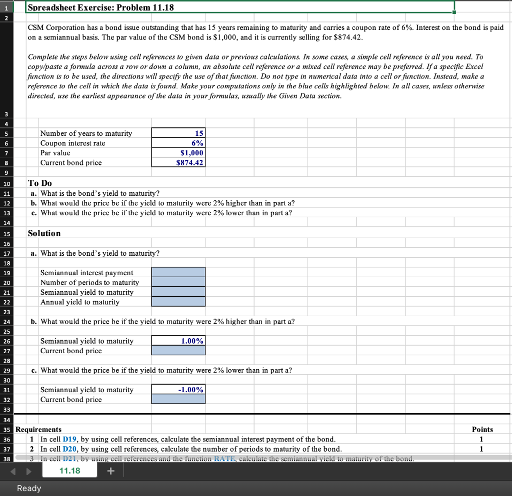

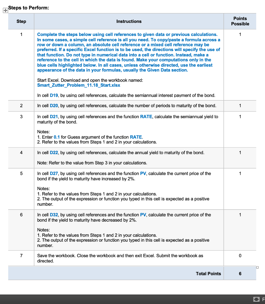
Spreadsheet Exercise: Problem 11.18 1 2 CSM Corporation has a bond issue outstanding that has 15 years remaining to maturity and carries a coupon rate of 6%. Interest on the bond is paid on a semiannual basis. The par value of the CSM bond is $1,000, and it is currently selling for $874.42. Complete the steps below using cell references to given data or previous calculations. In some cases, a simple cell reference is all you need. To copy/paste a formula across a row or down a column, an absolute cell reference or a mixed cell reference may be preferred. If a specific Excel function is to be used, the directions will specify the use of that function. Do not type in numerical data into a cell or function. Instead, make a reference to the cell in which the data is found. Make your computations only in the blue cells highlighted below. In all cases, unless otherwise directed, use the earliest appearance of the data in your formulas, usually the Given Data section. 5 6 7 Number of years to maturity Coupon interest rate Par value Current bond price 15 6% $1,000 $874.42 8 9 10 11 To Do a. What is the bond's yield to maturity? b. What would the price be if the yield to maturity were 2% higher than in part a? c. What would the price be if the yield to maturity were 2% lower than in part a? 12 13 14 15 Solution a. What is the bond's yield to maturity? 16 17 18 19 20 21 22 Semiannual interest payment Number of periods to maturity Semiannual yield to maturity Annual yield to maturity 23 24 b. What would the price be if the yield to maturity were 2% higher than in part a? 25 26 1.00% Semiannual yield to maturity Current bond price 27 28 29 c. What would the price be if the yield to maturity were 2% lower than in part a? 30 -1.00% 31 32 33 Semiannual yield to maturity Current bond price 34 35 Requirements 36 1 In cell D19, by using cell references, calculate the semiannual interest payment of the bond. 2 In cell D20, by using cell references, calculate the number of periods to maturity of the bond. 3 In cell D21, by using cell references and the function RATE, calculate the semiannual yield to maturity of the bond. 11.18 Points 1 1 37 38 + Ready Steps to Perform: Step Instructions Points Possible 1 1 Complete the steps below using cell references to given data or previous calculations. In some cases, a simple cell reference is all you need. To copy/paste a formula across a row or down a column, an absolute cell reference or a mixed cell reference may be preferred. If a specific Excel function is to be used, the directions will specify the use of that function. Do not type in numerical data into a cell or function. Instead, make a reference to the cell in which the data is found. Make your computations only in the blue cells highlighted below. In all cases, unless otherwise directed, use the earliest appearance of the data in your formulas, usually the Given Data section. Start Excel. Download and open the workbook named: Smart_Zutter_Problem_11.18_Start.xlsx In cell D19, by using cell references, calculate the semiannual interest payment of the bond. 2 In cell D20, by using cell references, calculate the number of periods to maturity of the bond. 1 3 1 In cell D21, by using cell references and the function RATE, calculate the semiannual yield to maturity of the bond. Notes: 1. Enter 0.1 for Guess argument of the function RATE. 2. Refer to the values from Steps 1 and 2 in your calculations. 4 In cell D22, by using cell references, calculate the annual yield to maturity of the bond. 1 Note: Refer to the value from Step 3 in your calculations. 5 1 In cell D27, by using cell references and the function PV, calculate the current price of the bond if the yield to maturity have increased by 2%. Notes: 1. Refer to the values from Steps 1 and 2 in your calculations. 2. The output of the expression or function you typed in this cell is expected as a positive number. 6 1 In cell D32, by using cell references and the function PV, calculate the current price of the bond if the yield to maturity have decreased by 2%. Notes: 1. Refer to the values from Steps 1 and 2 in your calculations. 2. The output of the expression or function you typed in this cell is expected as a positive number. 7 0 Save the workbook. Close the workbook and then exit Excel. Submit the workbook as directed. Total Points 6 F