Please

help with questions 1, and make sure codes work on R Studios.

Consider a location (locus) in the genome of a diploid organism where two different versions (alleles) of the DNA exist in the population. In particular, we can imagine that some copies of the locus have an adenine (A) and others have a thymine (T). We are interested in the frequency of adenine (A) alleles at the locus. It is possible under some assumptions to show that the frequency of the A allele has a stationary distribution. We do not have enough probability theory to define the idea of a stationary distribution rigorously, but we might describe it in this case as a distribution of the allele frequencies we would observe if we checked on the locus at widely separated times over a long period of evolution. We will use the stationary distribution as a prior distribution for , the frequency of the A allele.

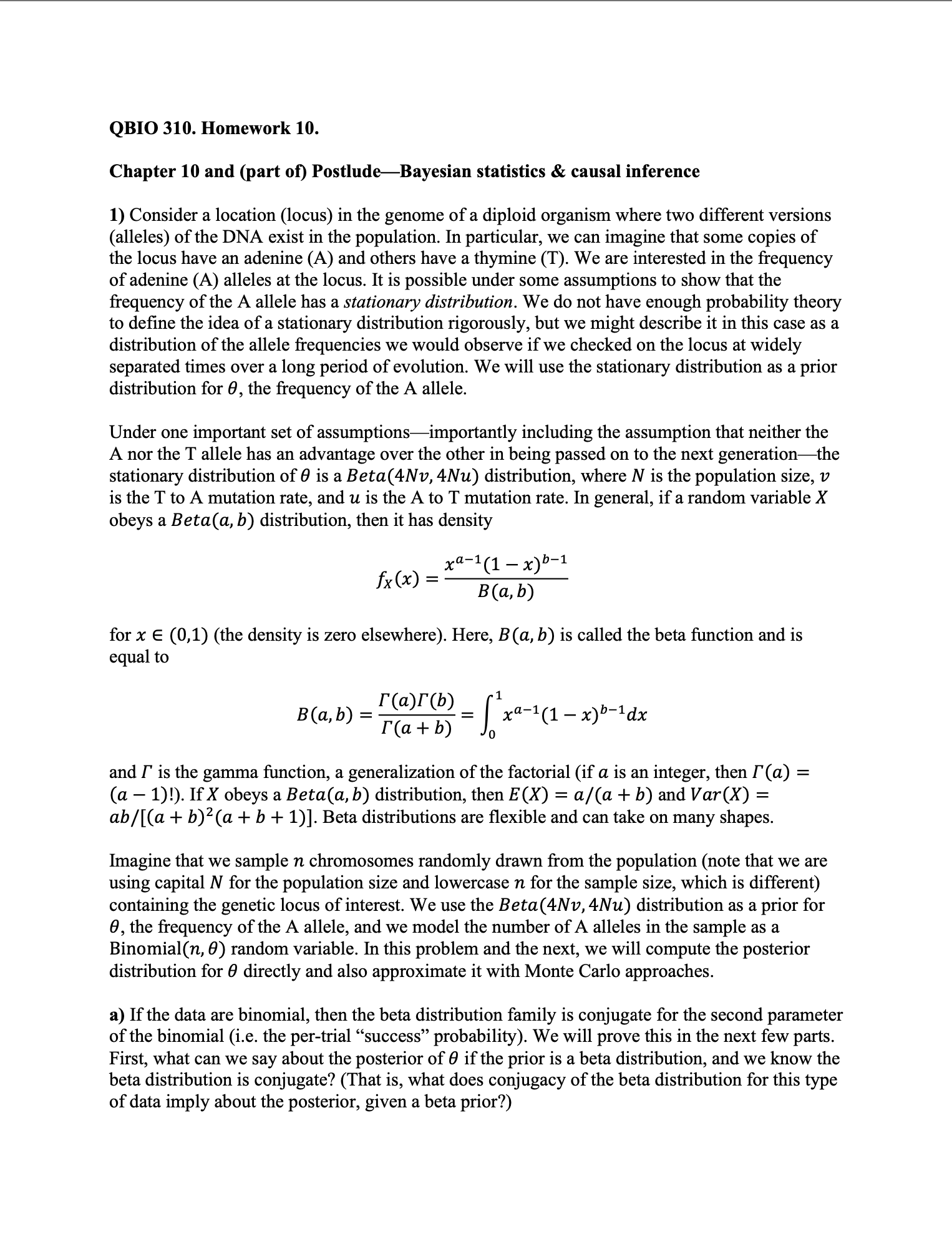
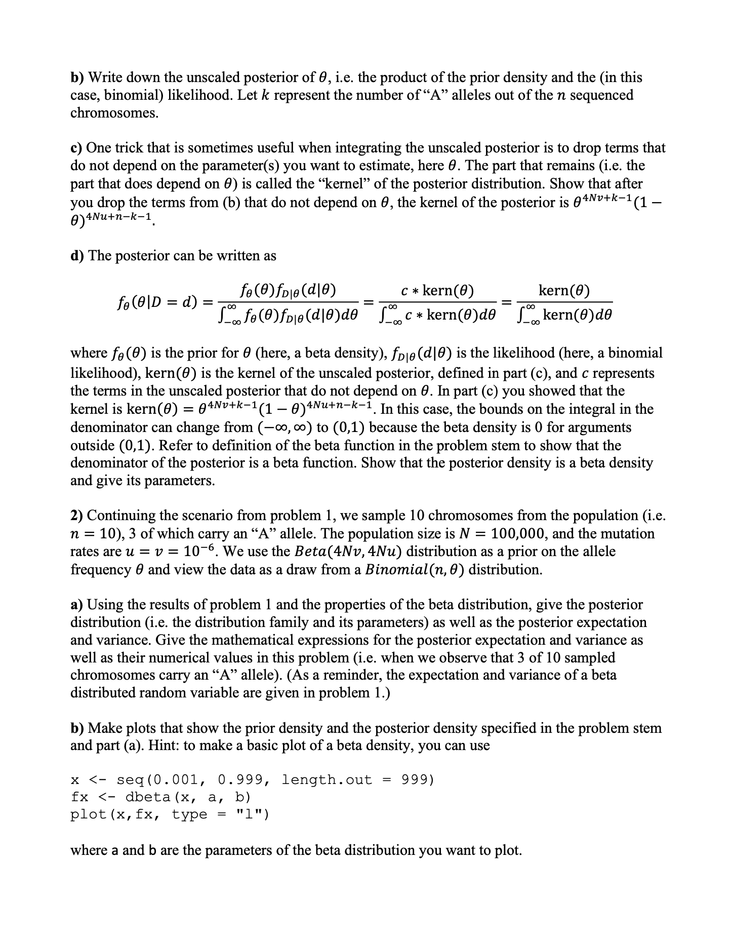
QBIO 310. Homework 10. Chapter 10 and (part of) PostludeBayesian statistics & causal inference 1) Consider a location (locus) in the genome of a diploid organism where two different versions (alleles) of the DNA exist in the population. In particular, we can imagine that some copies of the locus have an adenine (A) and others have a thymine (T). We are interested in the frequency of adenine (A) alleles at the locus. It is possible under some assumptions to show that the frequency of the A allele has a stationary distribution. We do not have enough probability theory to dene the idea of a stationary distribution rigorously, but we might describe it in this case as a distribution of the allele 'equencies we would observe if we checked on the locus at widely separated times over a long period of evolution. We will use the stationary distribution as a prior distribution for 9, the frequency of the A allele. Under one important set of assumptionsimportantly including the assumption that neither the A nor the T allele has an advantage over the other in being passed on to the next generationthe stationary distribution of 9 is a Beta(4Nv, 4Nu) distribution, where N is the population size, 1.7 is the T to A mutation rate, and u is the A to T mutation rate. In general, if a random variable X obeys a Beta(a, 1)) distribution, then it has density xa1(1 _ x)b1 am: 3%\" for x E (0,1) (the density is zero elsewhere). Here, B(a, b) is called the beta function and is equal to _ F(a)F(b) _ 1 _ _ al 1 _ b1d r(a + b) I, x C x) x B(a, b) and F is the gamma function, a generalization of the factorial (if a is an integer, then F(a) = (a 1)!) IfX obeys a Beta(a, 1)) distribution, then E(X) = a/(a + b) and Var(X) = ab / [(a + b)2(a + b + 1)]. Beta distributions are exible and can take on many shapes. Imagine that we sample 11 chromosomes randomly drawn from the population (note that we are using capital N for the population size and lowercase n for the sample size, which is different) containing the genetic locus of interest. We use the Beta (4N1), 4N u) distribution as a prior for 9, the frequency of the A allele, and we model the number of A alleles in the sample as a Binomia1(n, 9) random variable. In this problem and the next, we will compute the posterior distribution for 9 directly and also approximate it with Monte Carlo approaches. a) If the data are binomial, then the beta distribution family is conjugate for the second parameter of the binomial (i.e. the pertrial \"success\" probability). We will prove this in the next few parts. First, what can we say about the posterior of 9 if the prior is a beta distribution, and we know the beta distribution is conjugate? (That is, what does conjugacy of the beta distribution for this type of data imply about the posterior, given a beta prior?) b) Write down the unscaled posterior of 9, Le. the product of the prior density and the (in this case, binomial) likelihood. Let k represent the number of \"A\" alleles out of the n sequenced chromosomes. c) One trick that is sometimes useful when integrating the unscaled posterior is to drop terms that do not depend on the parameter(s) you want to estimate, here 9. The part that remains (i.e. the part that does depend on 9) is called the \"kernel\" of the posterior distribution. Show that after you drop the terms from (b) that do not depend on B, the kernel of the posterior is B4Nv+k'1 (1 9)4Nu+nk1l d) The posterior can be written as f3 (9)fplg(dl9) c * kern(6) kern(9) few = d) = W = time . kernww Z W where f9 (9) is the prior for 6 (here, a beta density), fDIQ (tilt?) is the likelihood (here, a binomial likelihood), kern(9) is the kernel of the unscaled posterior, dened in part (c), and C represents the terms in the unscaled posterior that do not depend on 9. In part (c) you showed that the kernel is kern(3) = 94Nv+k'1(1 9)4N\"+"'k'1. In this case, the bounds on the integral in the denominator can change from (00, 00) to (0,1) because the beta density is O for arguments outside (0,1). Refer to denition of the beta function in the problem stem to show that the denominator of the posterior is a beta function. Show that the posterior density is a beta density and give its parameters. 2) Continuing the scenario from problem 1, we sample 10 chromosomes from the population (i.e. n = 10), 3 of which carry an \"A\" allele. The population size is N = 100,000, and the mutation rates are u = v = 106. We use the Beta(4Nv, 4Nu) distribution as a prior on the allele frequency 6 and view the data as a draw from a Binomiat(n, 9) distribution. 3) Using the results of problem 1 and the properties of the beta distribution, give the posterior distribution (i.e. the distribution family and its parameters) as well as the posterior expectation and variance. Give the mathematical expressions for the posterior expectation and variance as well as their numerical values in this problem (i.e. when we observe that 3 of 10 sampled chromosomes carry an \"A\" allele). (As a reminder, the expectation and variance of a beta distributed random variable are given in problem 1.) b) Make plots that show the prior density and the posterior density specied in the problem stem and part (a). Hint: to make a basic plot of a beta density, you can use x