Please help with the cell references. They are very tricky.

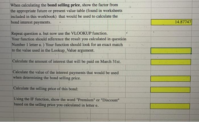
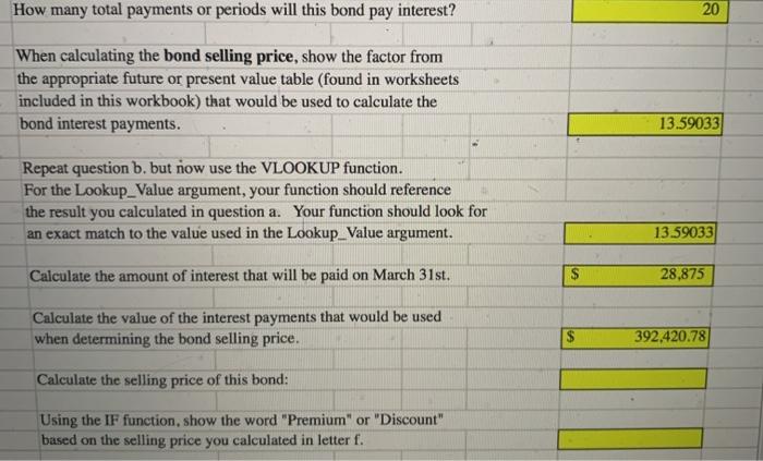
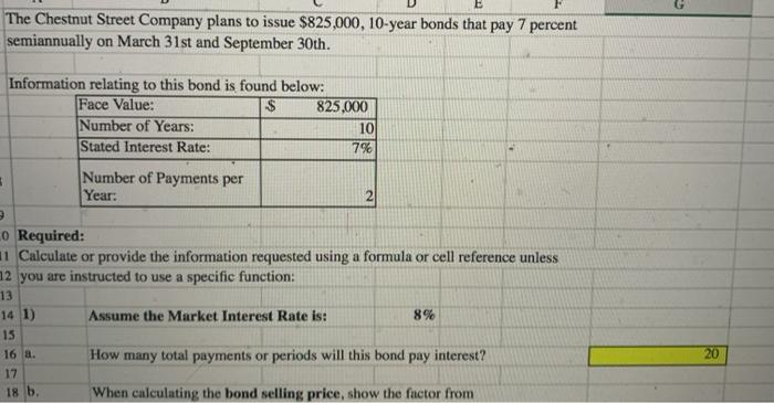
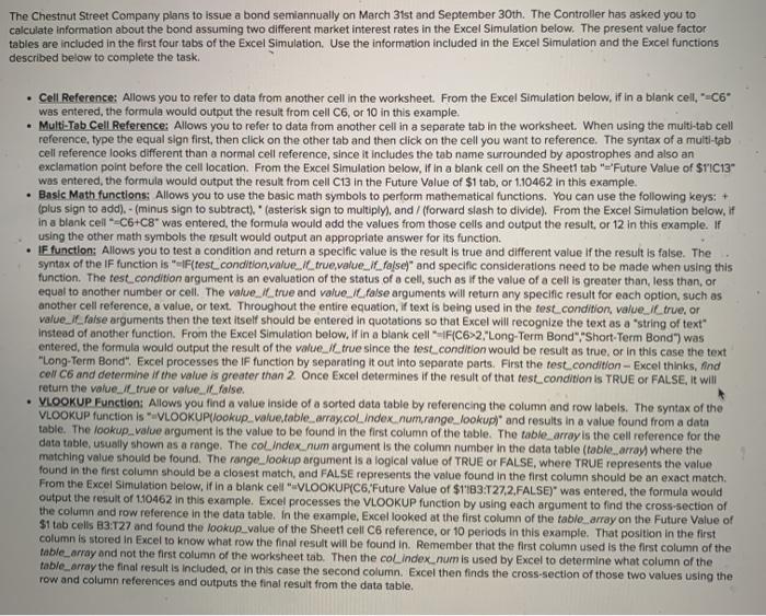
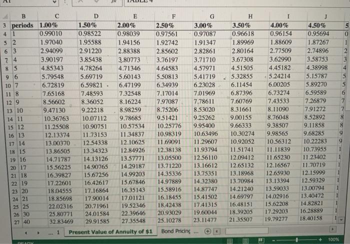
When calculating the bond selling price, show the factor from the appropriate future or present value table (found in worksheets included in this workbook) that would be used to calculate the bond interest payments. 14.87747 Repeat question a. but now use the VLOOKUP function. Your function should reference the result you calculated in question Number 1 letter a.) Your function should look for an exact match to the value used in the Lookup_value argument. Calculate the amount of interest that will be paid on March 31st. Calculate the value of the interest payments that would be used when determining the bond selling price. Calculate the selling price of this bond: Using the IF function, show the word "Premium" or "Discount" based on the selling price you calculated in letter e. How many total payments or periods will this bond pay interest? 20 When calculating the bond selling price, show the factor from the appropriate future or present value table (found in worksheets included in this workbook) that would be used to calculate the bond interest payments. 13.59033 Repeat question b. but now use the VLOOKUP function. For the Lookup_value argument, your function should reference the result you calculated in question a. Your function should look for an exact match to the value used the Lookup_value argument. 13.59033 Calculate the amount of interest that will be paid on March 31st. $ 28,875 Calculate the value of the interest payments that would be used when determining the bond selling price. 392,420.78 Calculate the selling price of this bond: Using the IF function, show the word "Premium" or "Discount" based on the selling price you calculated in letter f. The Chestnut Street Company plans to issue $825,000, 10-year bonds that pay 7 percent semiannually on March 31st and September 30th. Information relating to this bond is found below: Face Value: 825,000 Number of Years: 10 Stated Interest Rate: 7% Number of Payments per Year: 2 Lo Required: 1 Calculate or provide the information requested using a formula or cell reference unless 12 you are instructed to use a specific function: 13 14 1) Assume the Market Interest Rate is: 8% 15 16 a. How many total payments or periods will this bond pay interest? 17 When calculating the bond selling price, show the factor from 20 18 b, The Chestnut Street Company plans to issue a bond semiannually on March 31st and September 30th. The Controller has asked you to calculate information about the bond assuming two different market interest rates in the Excel Simulation below. The present value factor tables are included in the first four tabs of the Excel Simulation. Use the information included in the Excel Simulation and the Excel functions described below to complete the task. Cell Reference: Allows you to refer to data from another cell in the worksheet. From the Excel Simulation below, if in a blank ceil. --C6 was entered the formula would output the result from cell C6 or 10 in this example, Multi-Tab Cell Reference: Allows you to refer to data from another cell in a separate tab in the worksheet. When using the multi-tab cell reference, type the equal sign first, then click on the other tab and then click on the cell you want to reference. The syntax of a multi-tab cell reference looks different than a normal cell reference, since it includes the tab name surrounded by apostrophes and also an exclamation point before the cell location. From the Excel Simulation below, if in a blank cell on the Sheet1 tab "="Future Value of STIC13 was entered the formula would output the result from cell C13 in the Future Value of $1 tab, or 110462 in this example. Basic Math functions: Allows you to use the basic math symbols to perform mathematical functions. You can use the following keys: + (plus sign to add).- (minus sign to subtract) . * (asterisk sign to multiply), and / (forward slash to divide). From the Excel Simulation below, if in a blank cell-C6+C8" was entered the formula would add the values from those cells and output the result, or 12 In this example. If using the other math symbols the result would output an appropriate answer for its function. IF function: Allows you to test a condition and return a specific value is the result is true and different value if the result is false. The syntax of the IF function is "IF(test_condition value./_true,value_l lose)" and specific considerations need to be made when using this function. The test_condition argument is an evaluation of the status of a cell, such as if the value of a cell is greater than, less than, or equal to another number or cell. The value. Il true and value_/false arguments will return any specific result for each option, such as another cell reference, a value, or text. Throughout the entire equation, if text is being used in the test.condition, value Il true, or value_il_false arguments then the text itself should be entered in quotations so that Excel will recognize the text as a string of text instead of another function. From the Excel Simulation below, if in a blank cell -1FC6>2,"Long-Term Bond","Short-Term Bond") was entered the formula would output the result of the value_/l_true since the test condition would be result as true, or in this case the text "Long-Term Bond". Excel processes the IF function by separating it out into separate parts. First the test condition - Excel thinks, and Coll C6 and determine if the value is greater than 2 Once Excel determines if the result of that test.condition is TRUE OR FALSE, it will return the value true or value false. VLOOKUP Function: Allows you find a value inside of a sorted data table by referencing the column and row labels. The syntax of the VLOOKUP function is * VLOOKUP(lookup_value.table_array.col_index.num.range_lookup)" and results in a value found from a data table. The lookup_value argument is the value to be found in the first column of the table. The table_array is the cell reference for the data table, usually shown as a range. The colindex_num argument is the column number in the data table (table array) where the matching value should be found. The range, Jookup argument is a logical value of TRUE or FALSE, where TRUE represents the value found in the first column should be a closest match, and FALSE represents the value found in the first column should be an exact match, From the Excel Simulation below, if in a blank cel"VLOOKUP(C6, Future Value of $1183 T27,2,FALSE)" was entered the formula would output the result of 1.10462 in this example. Excel processes the VLOOKUP function by using each argument to find the cross-section of the column and row reference in the data table. In the example, Excel looked at the first column of the table array on the Future Value of $1 tab cells B3:127 and found the lookup_value of the Sheet cell C6 reference, or 10 periods in this example. That position in the first column is stored in Excel to know what row the final result will be found in. Remember that the first column used is the first column of the table_array and not the first column of the worksheet tab. Then the colindex_num is used by Excel to determine what column of the table_array the final result is included, or in this case the second column. Excel then finds the cross-section of those two values using the row and column references and outputs the final result from the data table, 0 - . + B D E 3 periods 1.00% 1.50% 2.00% 41 0.99010 0.98522 0.98039 52 1.97040 1.95588 1.94156 6 3 2.94099 291220 2.88388 74 3.90197 3.85438 3.80773 8 S 4.85343 4.78264 4.71346 9 6 5.79548 5.69719 5.60143 10 7 6.72819 6.59821 6.47199 11 8 7.65168 7.48593 7.32548 129 8.56602 8.36052 8.16224 13 10 9.47130 9.22218 8.98259 14 11 10.36763 10.07112 9.78685 15 12 11.25508 10.90751 10.57534 16 13 12.13374 11.73153 11.34837 17 14 13.00370 12.54338 12.10625 18 15 13.86505 13.34323 12.84926 19 16 14.71787 14.13126 13.57771 20 17 15 56225 14.90765 14.29187 21 18 16.39827 15.67256 14.99203 22 19 17.22601 16.42617 15.67846 23 20 18.04555 17.16864 16.35143 24 21 18.85698 17.90014 17.01121 25 25 22.02316 20.71961 19.52346 26 30 25.80771 24.01584 22.39646 27 40 32.83469 29.91585 27.35548 1 Present Value of Annuity of $1 F 2.50% 0.97561 1.92742 2.85602 3.76197 4.64583 5.50813 6.34939 7.17014 7.97087 8.75206 9.51421 10.25776 10.98319 11.69091 12.38138 13.05500 13.71220 14.35336 14.97889 15.58916 16.18455 18.42438 20.93029 25.10278 G 3.00% 0.97087 1.91347 2.82861 3.71710 4.57971 5.41719 6.23028 7.01969 7.78611 8.53020 9.25262 9.95400 10.63496 11.29607 11.93794 12.56110 13.16612 13.75351 14.32380 14.87747 15.41502 17.41315 19.60044 23.11477 H 3.50% 0.96618 1.89969 2.80164 3.67308 4.51505 5.32855 6.11454 6.87396 7.60769 8.31661 9.00155 9.66333 10.30274 10.92052 11.51741 12.09412 12.65132 13.18968 13.70984 14.21240 14.69797 16.48151 18.39205 21.35507 4.00% 0.96154 1.88609 2.77509 3.62990 4.45182 5.24214 6.00205 6.73274 7.43533 8.11090 8.76048 9.38507 9.98565 10.56312 11.11839 11.65230 12.16567 12.65930 13.13394 13.59033 14.02916 15.62208 17.29203 19.79277 J 4.50% 0.95694 1.87267 2.74896 3.58753 4.38998 5.15787 5.89270 6.59589 7.26879 791272 8.52892 9.11858 9.68285 10.22283 10.73955 11.23402 11.70719 12.15999 12.59329 13.00794 13.40472 14.82821 16.28889 18.40158 8 Bond Pricing 4 100% DAO When calculating the bond selling price, show the factor from the appropriate future or present value table (found in worksheets included in this workbook) that would be used to calculate the bond interest payments. 14.87747 Repeat question a. but now use the VLOOKUP function. Your function should reference the result you calculated in question Number 1 letter a.) Your function should look for an exact match to the value used in the Lookup_value argument. Calculate the amount of interest that will be paid on March 31st. Calculate the value of the interest payments that would be used when determining the bond selling price. Calculate the selling price of this bond: Using the IF function, show the word "Premium" or "Discount" based on the selling price you calculated in letter e. How many total payments or periods will this bond pay interest? 20 When calculating the bond selling price, show the factor from the appropriate future or present value table (found in worksheets included in this workbook) that would be used to calculate the bond interest payments. 13.59033 Repeat question b. but now use the VLOOKUP function. For the Lookup_value argument, your function should reference the result you calculated in question a. Your function should look for an exact match to the value used the Lookup_value argument. 13.59033 Calculate the amount of interest that will be paid on March 31st. $ 28,875 Calculate the value of the interest payments that would be used when determining the bond selling price. 392,420.78 Calculate the selling price of this bond: Using the IF function, show the word "Premium" or "Discount" based on the selling price you calculated in letter f. The Chestnut Street Company plans to issue $825,000, 10-year bonds that pay 7 percent semiannually on March 31st and September 30th. Information relating to this bond is found below: Face Value: 825,000 Number of Years: 10 Stated Interest Rate: 7% Number of Payments per Year: 2 Lo Required: 1 Calculate or provide the information requested using a formula or cell reference unless 12 you are instructed to use a specific function: 13 14 1) Assume the Market Interest Rate is: 8% 15 16 a. How many total payments or periods will this bond pay interest? 17 When calculating the bond selling price, show the factor from 20 18 b, The Chestnut Street Company plans to issue a bond semiannually on March 31st and September 30th. The Controller has asked you to calculate information about the bond assuming two different market interest rates in the Excel Simulation below. The present value factor tables are included in the first four tabs of the Excel Simulation. Use the information included in the Excel Simulation and the Excel functions described below to complete the task. Cell Reference: Allows you to refer to data from another cell in the worksheet. From the Excel Simulation below, if in a blank ceil. --C6 was entered the formula would output the result from cell C6 or 10 in this example, Multi-Tab Cell Reference: Allows you to refer to data from another cell in a separate tab in the worksheet. When using the multi-tab cell reference, type the equal sign first, then click on the other tab and then click on the cell you want to reference. The syntax of a multi-tab cell reference looks different than a normal cell reference, since it includes the tab name surrounded by apostrophes and also an exclamation point before the cell location. From the Excel Simulation below, if in a blank cell on the Sheet1 tab "="Future Value of STIC13 was entered the formula would output the result from cell C13 in the Future Value of $1 tab, or 110462 in this example. Basic Math functions: Allows you to use the basic math symbols to perform mathematical functions. You can use the following keys: + (plus sign to add).- (minus sign to subtract) . * (asterisk sign to multiply), and / (forward slash to divide). From the Excel Simulation below, if in a blank cell-C6+C8" was entered the formula would add the values from those cells and output the result, or 12 In this example. If using the other math symbols the result would output an appropriate answer for its function. IF function: Allows you to test a condition and return a specific value is the result is true and different value if the result is false. The syntax of the IF function is "IF(test_condition value./_true,value_l lose)" and specific considerations need to be made when using this function. The test_condition argument is an evaluation of the status of a cell, such as if the value of a cell is greater than, less than, or equal to another number or cell. The value. Il true and value_/false arguments will return any specific result for each option, such as another cell reference, a value, or text. Throughout the entire equation, if text is being used in the test.condition, value Il true, or value_il_false arguments then the text itself should be entered in quotations so that Excel will recognize the text as a string of text instead of another function. From the Excel Simulation below, if in a blank cell -1FC6>2,"Long-Term Bond","Short-Term Bond") was entered the formula would output the result of the value_/l_true since the test condition would be result as true, or in this case the text "Long-Term Bond". Excel processes the IF function by separating it out into separate parts. First the test condition - Excel thinks, and Coll C6 and determine if the value is greater than 2 Once Excel determines if the result of that test.condition is TRUE OR FALSE, it will return the value true or value false. VLOOKUP Function: Allows you find a value inside of a sorted data table by referencing the column and row labels. The syntax of the VLOOKUP function is * VLOOKUP(lookup_value.table_array.col_index.num.range_lookup)" and results in a value found from a data table. The lookup_value argument is the value to be found in the first column of the table. The table_array is the cell reference for the data table, usually shown as a range. The colindex_num argument is the column number in the data table (table array) where the matching value should be found. The range, Jookup argument is a logical value of TRUE or FALSE, where TRUE represents the value found in the first column should be a closest match, and FALSE represents the value found in the first column should be an exact match, From the Excel Simulation below, if in a blank cel"VLOOKUP(C6, Future Value of $1183 T27,2,FALSE)" was entered the formula would output the result of 1.10462 in this example. Excel processes the VLOOKUP function by using each argument to find the cross-section of the column and row reference in the data table. In the example, Excel looked at the first column of the table array on the Future Value of $1 tab cells B3:127 and found the lookup_value of the Sheet cell C6 reference, or 10 periods in this example. That position in the first column is stored in Excel to know what row the final result will be found in. Remember that the first column used is the first column of the table_array and not the first column of the worksheet tab. Then the colindex_num is used by Excel to determine what column of the table_array the final result is included, or in this case the second column. Excel then finds the cross-section of those two values using the row and column references and outputs the final result from the data table, 0 - . + B D E 3 periods 1.00% 1.50% 2.00% 41 0.99010 0.98522 0.98039 52 1.97040 1.95588 1.94156 6 3 2.94099 291220 2.88388 74 3.90197 3.85438 3.80773 8 S 4.85343 4.78264 4.71346 9 6 5.79548 5.69719 5.60143 10 7 6.72819 6.59821 6.47199 11 8 7.65168 7.48593 7.32548 129 8.56602 8.36052 8.16224 13 10 9.47130 9.22218 8.98259 14 11 10.36763 10.07112 9.78685 15 12 11.25508 10.90751 10.57534 16 13 12.13374 11.73153 11.34837 17 14 13.00370 12.54338 12.10625 18 15 13.86505 13.34323 12.84926 19 16 14.71787 14.13126 13.57771 20 17 15 56225 14.90765 14.29187 21 18 16.39827 15.67256 14.99203 22 19 17.22601 16.42617 15.67846 23 20 18.04555 17.16864 16.35143 24 21 18.85698 17.90014 17.01121 25 25 22.02316 20.71961 19.52346 26 30 25.80771 24.01584 22.39646 27 40 32.83469 29.91585 27.35548 1 Present Value of Annuity of $1 F 2.50% 0.97561 1.92742 2.85602 3.76197 4.64583 5.50813 6.34939 7.17014 7.97087 8.75206 9.51421 10.25776 10.98319 11.69091 12.38138 13.05500 13.71220 14.35336 14.97889 15.58916 16.18455 18.42438 20.93029 25.10278 G 3.00% 0.97087 1.91347 2.82861 3.71710 4.57971 5.41719 6.23028 7.01969 7.78611 8.53020 9.25262 9.95400 10.63496 11.29607 11.93794 12.56110 13.16612 13.75351 14.32380 14.87747 15.41502 17.41315 19.60044 23.11477 H 3.50% 0.96618 1.89969 2.80164 3.67308 4.51505 5.32855 6.11454 6.87396 7.60769 8.31661 9.00155 9.66333 10.30274 10.92052 11.51741 12.09412 12.65132 13.18968 13.70984 14.21240 14.69797 16.48151 18.39205 21.35507 4.00% 0.96154 1.88609 2.77509 3.62990 4.45182 5.24214 6.00205 6.73274 7.43533 8.11090 8.76048 9.38507 9.98565 10.56312 11.11839 11.65230 12.16567 12.65930 13.13394 13.59033 14.02916 15.62208 17.29203 19.79277 J 4.50% 0.95694 1.87267 2.74896 3.58753 4.38998 5.15787 5.89270 6.59589 7.26879 791272 8.52892 9.11858 9.68285 10.22283 10.73955 11.23402 11.70719 12.15999 12.59329 13.00794 13.40472 14.82821 16.28889 18.40158 8 Bond Pricing 4 100% DAO