Please Leave clear step by step instructions with listed cells and formulas. Thank you!

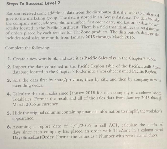
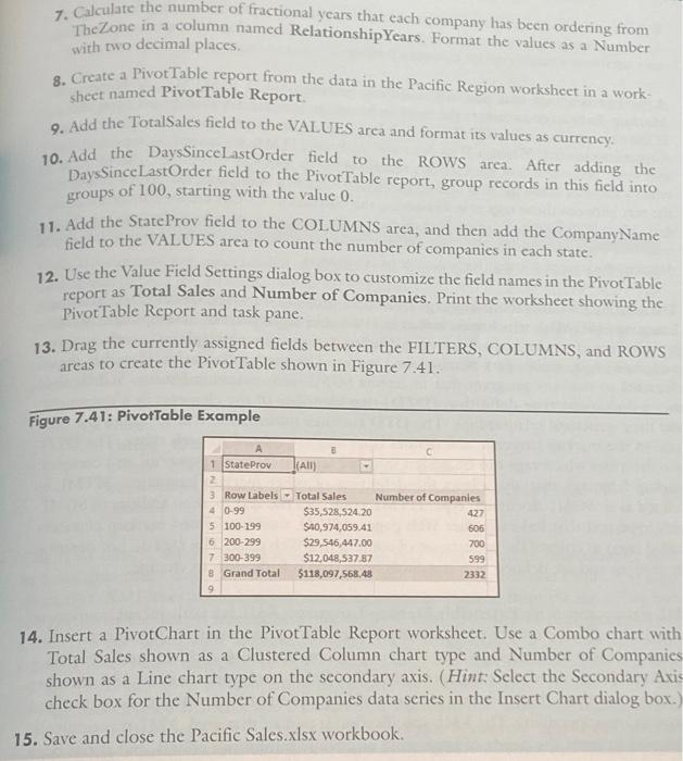
Barbara received some additional data from the distributor that she needs to analyze and give to the marketing group. The data is stored in an Access database. The data includes the company name, address, phone number, first order date, and last order date for cach retailer located in the Pacific Northwest. There is a field that identifies the total number of orders placed by each retailer for TheZone products. The distributor's database also includes total sales by month, from January 2015 through March 2016. Complete the following: 1. Create a new workbook, and save it as Pacific Sales.xlsx in the Chapter 7 folder. 2. Import the data contained in the Pacific Region table of the Pacific.accdb Access database located in the Chapter 7 folder into a worksheet named Pacific Region. 3. Sort the data first by state/province, then by city, and then by company name in ascending order. 4. Calculate the total sales since January 2015 for each company in a column labeled TotalSales. Format the result and all of the sales data from January 2015 through March 2016 as currency. 5. Hide the original columns containing financial information to simplify the worksheet's appearance. 6. Assuming a report date of 4/1/2016 in cell ACl, calculate the number of days since each company has placed an order with TheZone in a column named DaysSinceLastOrder. Format the values as a Number with zero decimal places. 7. Calculate the number of fractional years that each company has been ordering from TheZone in a column named RelationshipYears. Format the valtues as a Number with two decimat places. 8. Create a Pivot Table report from the data in the Pacific Region worksheet in a worksheet named PivotTable Report: 9. Add the Toralsales field to the VALUES area and format its values as currency. 10. Add the DaysSincelastOrder field to the ROWS area. After adding the Days SinceLastOrder field to the Pivot Table report, group records in this field into groups of 100 , starting with the value 0 . 11. Add the StateProv field to the COLUMNS area, and then add the CompanyName field to the VALUES area to count the number of companies in each state. 12. Use the Value Field Settings dialog box to customize the field names in the PivotTable report as Total Sales and Number of Companies. Print the worksheet showing the PivotTable Report and task pane: 13. Drag the currently assigned fields between the FILTERS, COLUMNS, and ROWS areas to create the Pivot Table shown in Figure 7.41. Figure 7.41: PivotTable Example 14. Insert a PivotChart in the PivotTable Report worksheet. Use a Combo chart with Total Sales shown as a Clustered Column chart type and Number of Companie shown as a Line chart type on the secondary axis. (Hint: Seleet the Secondary Axi check box for the Number of Companies data series in the Insert Chart dialog box. 15. Save and close the Pacific Sales.xlsx workbook