

Question: please only answer 4. I included 1 and 2 because you use them to answer 4 Sheet 2: c n= 20 I= 2% Cash Flows
please only answer 4. I included 1 and 2 because you use them to answer 4 Sheet 2: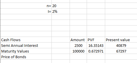

 c
c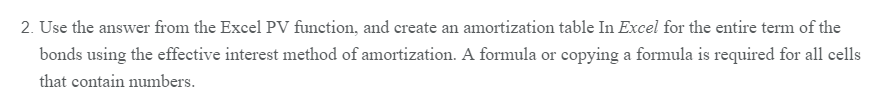
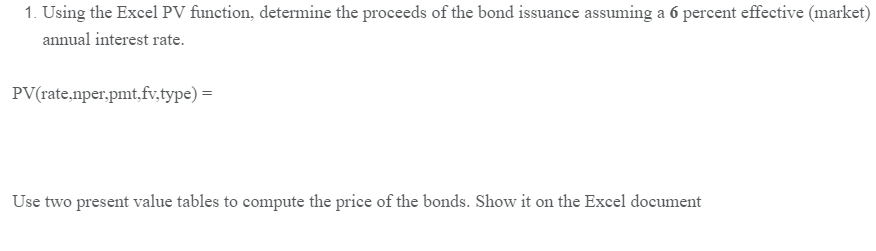
n= 20 I= 2% Cash Flows Semi Annual Interest Maturity Values Price of Bonds Amount PVF Present value 2500 16.35143 40879 100000 0.672971 67297 On January 1, 2018, the Blue Devil Corporation issued $100,000 of ten-year bonds. The bonds carried a stated annual interest rate of 5 percent, with interest payable semiannually on June 30 and December 31. 1. Using the Excel PV function, determine the proceeds of the bond issuance assuming a 6 percent effective (market) annual interest rate. PV(rate,nper,pmt,fv.type) = Use two present value tables to compute the price of the bonds. Show it on the Excel document 4. Using sheet 2 of the same file you created for step 2, repeat step 2 above assuming that the market annual interest rate is 4 percent. 2. Use the answer from the Excel PV function, and create an amortization table In Excel for the entire term of the bonds using the effective interest method of amortization. A formula or copying a formula is required for all cells that contain numbers
Step by Step Solution
There are 3 Steps involved in it

Get step-by-step solutions from verified subject matter experts