please please help!

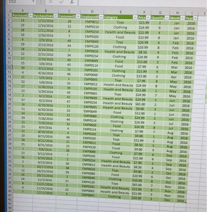
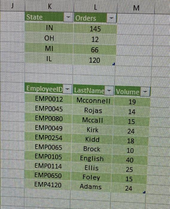
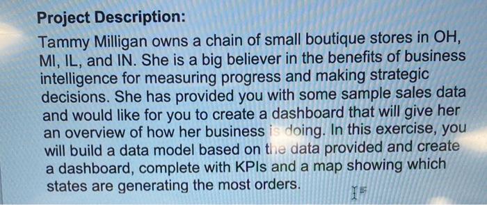
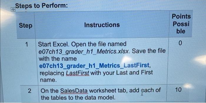
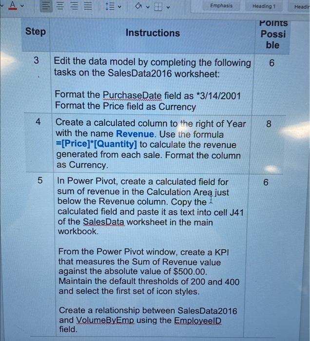
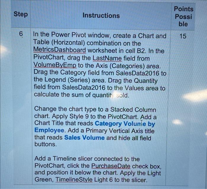
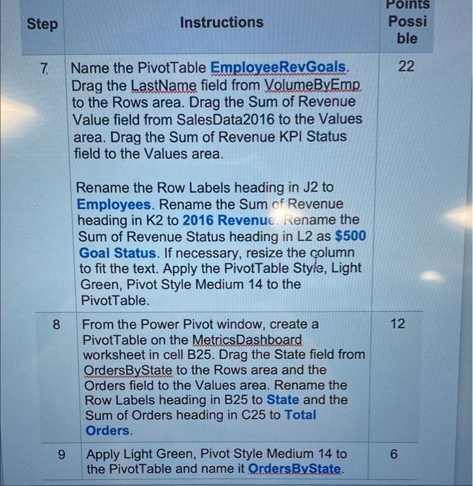
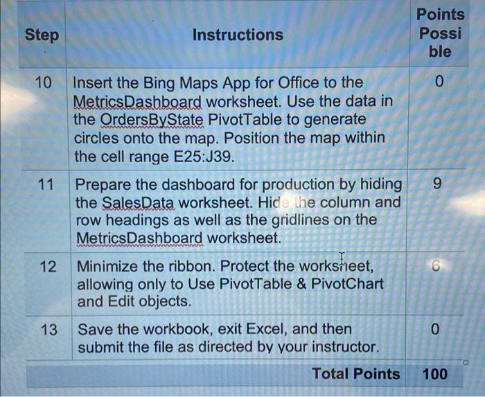
012 So > for - Nm G Quantity 2 9 4 8 Toys 6 8 4 9 3 6 9 3 8 H Month Jan Jan Jan Jan Feb Feb Feb Feb Feb Mar Mar Apr May May May 00 May B PurchaseDate Customer 1/13/2016 28 1/14/2016 12 1/21/2016 8 1/30/2016 7 2/9/2016 49 2/13/2016 34 2/14/2016 7 2/15/2016 34 2/19/2016 49 3/8/2016 43 3/12/2016 31 4/16/2016 46 5/4/2016 1 5/8/2016 35 5/28/2016 39 5/29/2016 43 6/2/2016 42 6/2/2016 47 6/19/2016 6/20/2016 33 6/21/2016 15 7/28/2016 44 7/29/2016 32 8/9/2016 4 8/10/2016 4 8/13/2016 46 8/22/2016 21 8/31/2016 25 9/8/2016 38 9/12/2016 7 9/24/2016 2 9/25/2016 30 10/17/2016 38 10/23/2016 39 10/23/2016 3 11/3/2016 21 11/21/2016 2 11/24/2016 32 12/11/2016 4 1 Purchased 14 3 19 28 10 6 9 7 29 8 18 9 22 10 27 11 25 12 30 33 4 14 21 15 32 16 17 17 13 18 2 19 37 20 16 21 11 22 34 23 39 24 15 25 33 26 31 27 20 28 38 29 35 30 1 31 23 32 36 33 3 34 5 35 12 36 26 37 24 38 8 39 6 40 7 41 42 43 44 D Employeeld EMPO012 EMP0114 EMPO254 EMP0105 EMP0049 EMP4120 EMP0650 EMPO254 EMP0049 EMP0114 EMPO105 EMP0049 EMP0045 EMPO012 EMPO105 EMPO065 EMPO049 EMPO254 EMP0045 EMP0049 EMPO080 EMPO114 EMP0650 EMPO114 EMPO 105 EMPO105 EMPO012 EMP4120 EMPO080 EMPO105 EMPO254 EMP0012 EMP0650 EMPOOBO EMPO049 EMP4120 EMPO 105 EMPO065 EMP0045 8 1 7 3 2 E F Category Price Toys $15.99 Clothing $24.99 Health and Beauty $15.99 Food $15.99 $24.99 Clothing $10.99 Health and Beauty $8.50 Clothing $24.99 Food $13.00 Food 57.99 Clothing $15.99 Clothing $13.00 Toys $7.99 Health and Beauty 524.99 Health and Beauty $12.00 Toys $24.99 Health and Beauty S24.99 Health and Beauty S65.00 Health and Beauty59.00 Food $12.00 Clothing $24.99 Clothing 2499 Food $24.99 Clothing $7.99 Toys $9.00 Toys $15.99 Food $8.50 Food 59.00 Clothing $7.99 Food $15.99 Health and Beauty: $7.99 Health and Beauty S8 50 Toys $9.00 Food $10.99 Clothing $10.99 $65.00 Health and Beauty $15.99 Health and Beauty $15.99 Clothing $24.99 3 1 3 3 8 7 5 2 5 9 6 6 3 4 3 6 8 7 9 Jun Jun Jun Jun Jun Jul Jul Aug Aug Aug Aug Aug Sep Sep Sep Sep Oct Oct Oct Nov Dec Year 2016 2016 2016 2016 2016 2016 2016 2016 2016 2016 2016 2016 2016 2016 2016 2016 2016 2016 2016 2016 2016 2016 2016 2016 2016 2016 2016 2016 2016 2016 2016 2016 2016 2016 2016 2016 2016 2016 2016 Toys LOOM 3 K L M 1 Orders State IN 145 12 OH MI 66 120 Employees EMP0012 EMP0045 EMPO080 EMP0049 EMPO254 EMPO065 EMPO105 EMPO114 EMP0650 EMP4120 LastName - Volume Mcconnell 19 Rojas Mccall 15 Kirk 24 Kidd Brock 10 English 40 Ellis 25 Foley Adams 24 Description Workbook Name e07ch 13Metrics.xlsx Last Version Backup Name Mod. Description 4 5 Create Date By Whom 6 mm/dd/yyyy Firstname Lastname 7 Mod. Date By Whom 8 9 10 11 12 13 14 15 16 17 18 19 Create Date Sheet Name 20 21 22 23 Creator Purpose Project Description: Tammy Milligan owns a chain of small boutique stores in OH, MI, IL, and IN. She is a big believer in the benefits of business intelligence for measuring progress and making strategic decisions. She has provided you with some sample sales data and would like for you to create a dashboard that will give her an overview of how her business is doing. In this exercise, you will build a data model based on the data provided and create a dashboard, complete with KPls and a map showing which states are generating the most orders. Steps to Perform: Step Instructions Points Possi ble 1 0 Start Excel. Open the file named e07ch13 grader_h1_Metrics.xlsx. Save the file with the name e07ch13_grader_h1_Metrics_LastFirst, replacing LastFirst with your Last and First name. On the SalesData worksheet tab, add pach of the tables to the data model. 2 10 - Av Emphasis Heading 1 Headir Step Instructions Points Possi ble 3 Edit the data model by completing the following tasks on the Sales Data 2016 worksheet: 6 4 8 Format the Purchase Date field as *3/14/2001 Format the Price field as Currency Create a calculated column to the right of Year with the name Revenue. Use the formula =[Price]*[Quantity] to calculate the revenue generated from each sale. Format the column as Currency. In Power Pivot, create a calculated field for sum of revenue in the Calculation Area just below the Revenue column. Copy the calculated field and paste it as text into cell J41 of the SalesData worksheet in the main workbook 5 6 6 From the Power Pivot window, create a KPI that measures the Sum of Revenue value against the absolute value of $500.00. Maintain the default thresholds of 200 and 400 and select the first set of icon styles. Create a relationship between Sales Data 2016 and VolumeByEmp using the Employeeld field. Step Instructions Points Possi ble 6 15 In the Power Pivot window, create a Chart and Table (Horizontal) combination on the Metrics Dashboard worksheet in cell B2. In the PivotChart, drag the LastName field from VolumeByEmp to the Axis (Categories) area. Drag the Category field from Sales Data 2016 to the Legend (Series) area. Drag the Quantity field from Sales Data 2016 to the Values area to calculate the sum of quantit sold. Change the chart type to a Stacked Column chart. Apply Style 9 to the PivotChart. Add a Chart Title that reads Category Volume by Employee. Add a Primary Vertical Axis title that reads Sales Volume and hide all field buttons. Add a Timeline slicer connected to the PivotChart, click the PurchaseDate check box, and position it below the chart. Apply the Light Green, Timeline Style Light 6 to the slicer. Step Instructions Points Possi ble 7 22 Name the Pivot Table Employee RevGoals. Drag the LastName field from VolumeByEmp to the Rows area. Drag the Sum of Revenue Value field from Sales Data 2016 to the Values area. Drag the Sum of Revenue KPI Status field to the Values area. 8 Rename the Row Labels heading in J2 to Employees. Rename the Sum of Revenue heading in K2 to 2016 Revenue. Rename the Sum of Revenue Status heading in L2 as $500 Goal Status. If necessary, resize the column to fit the text. Apply the PivotTable Style, Light Green, Pivot Style Medium 14 to the Pivot Table From the Power Pivot window, create a Pivot Table on the Metrics Dashboard worksheet in cell B25. Drag the State field from OrdersByState to the Rows area and the Orders field to the Values area. Rename the Row Labels heading in B25 to State and the Sum of Orders heading in C25 to Total Orders. Apply Light Green, Pivot Style Medium 14 to the Pivot Table and name it OrdersByState. 12 9 6 Step Instructions Points Possi ble 10 0 11 9 Insert the Bing Maps App for Office to the Metrics Dashboard worksheet. Use the data in the OrdersByState PivotTable to generate circles onto the map. Position the map within the cell range E25:39. Prepare the dashboard for production by hiding the SalesData worksheet. Hide the column and row headings as well as the gridlines on the Metrics Dashboard worksheet. Minimize the ribbon. Protect the worksheet, allowing only to Use PivotTable & PivotChart and Edit objects. Save the workbook, exit Excel, and then submit the file as directed by your instructor. 12 6 13 0 Total Points 100 012 So > for - Nm G Quantity 2 9 4 8 Toys 6 8 4 9 3 6 9 3 8 H Month Jan Jan Jan Jan Feb Feb Feb Feb Feb Mar Mar Apr May May May 00 May B PurchaseDate Customer 1/13/2016 28 1/14/2016 12 1/21/2016 8 1/30/2016 7 2/9/2016 49 2/13/2016 34 2/14/2016 7 2/15/2016 34 2/19/2016 49 3/8/2016 43 3/12/2016 31 4/16/2016 46 5/4/2016 1 5/8/2016 35 5/28/2016 39 5/29/2016 43 6/2/2016 42 6/2/2016 47 6/19/2016 6/20/2016 33 6/21/2016 15 7/28/2016 44 7/29/2016 32 8/9/2016 4 8/10/2016 4 8/13/2016 46 8/22/2016 21 8/31/2016 25 9/8/2016 38 9/12/2016 7 9/24/2016 2 9/25/2016 30 10/17/2016 38 10/23/2016 39 10/23/2016 3 11/3/2016 21 11/21/2016 2 11/24/2016 32 12/11/2016 4 1 Purchased 14 3 19 28 10 6 9 7 29 8 18 9 22 10 27 11 25 12 30 33 4 14 21 15 32 16 17 17 13 18 2 19 37 20 16 21 11 22 34 23 39 24 15 25 33 26 31 27 20 28 38 29 35 30 1 31 23 32 36 33 3 34 5 35 12 36 26 37 24 38 8 39 6 40 7 41 42 43 44 D Employeeld EMPO012 EMP0114 EMPO254 EMP0105 EMP0049 EMP4120 EMP0650 EMPO254 EMP0049 EMP0114 EMPO105 EMP0049 EMP0045 EMPO012 EMPO105 EMPO065 EMPO049 EMPO254 EMP0045 EMP0049 EMPO080 EMPO114 EMP0650 EMPO114 EMPO 105 EMPO105 EMPO012 EMP4120 EMPO080 EMPO105 EMPO254 EMP0012 EMP0650 EMPOOBO EMPO049 EMP4120 EMPO 105 EMPO065 EMP0045 8 1 7 3 2 E F Category Price Toys $15.99 Clothing $24.99 Health and Beauty $15.99 Food $15.99 $24.99 Clothing $10.99 Health and Beauty $8.50 Clothing $24.99 Food $13.00 Food 57.99 Clothing $15.99 Clothing $13.00 Toys $7.99 Health and Beauty 524.99 Health and Beauty $12.00 Toys $24.99 Health and Beauty S24.99 Health and Beauty S65.00 Health and Beauty59.00 Food $12.00 Clothing $24.99 Clothing 2499 Food $24.99 Clothing $7.99 Toys $9.00 Toys $15.99 Food $8.50 Food 59.00 Clothing $7.99 Food $15.99 Health and Beauty: $7.99 Health and Beauty S8 50 Toys $9.00 Food $10.99 Clothing $10.99 $65.00 Health and Beauty $15.99 Health and Beauty $15.99 Clothing $24.99 3 1 3 3 8 7 5 2 5 9 6 6 3 4 3 6 8 7 9 Jun Jun Jun Jun Jun Jul Jul Aug Aug Aug Aug Aug Sep Sep Sep Sep Oct Oct Oct Nov Dec Year 2016 2016 2016 2016 2016 2016 2016 2016 2016 2016 2016 2016 2016 2016 2016 2016 2016 2016 2016 2016 2016 2016 2016 2016 2016 2016 2016 2016 2016 2016 2016 2016 2016 2016 2016 2016 2016 2016 2016 Toys LOOM 3 K L M 1 Orders State IN 145 12 OH MI 66 120 Employees EMP0012 EMP0045 EMPO080 EMP0049 EMPO254 EMPO065 EMPO105 EMPO114 EMP0650 EMP4120 LastName - Volume Mcconnell 19 Rojas Mccall 15 Kirk 24 Kidd Brock 10 English 40 Ellis 25 Foley Adams 24 Description Workbook Name e07ch 13Metrics.xlsx Last Version Backup Name Mod. Description 4 5 Create Date By Whom 6 mm/dd/yyyy Firstname Lastname 7 Mod. Date By Whom 8 9 10 11 12 13 14 15 16 17 18 19 Create Date Sheet Name 20 21 22 23 Creator Purpose Project Description: Tammy Milligan owns a chain of small boutique stores in OH, MI, IL, and IN. She is a big believer in the benefits of business intelligence for measuring progress and making strategic decisions. She has provided you with some sample sales data and would like for you to create a dashboard that will give her an overview of how her business is doing. In this exercise, you will build a data model based on the data provided and create a dashboard, complete with KPls and a map showing which states are generating the most orders. Steps to Perform: Step Instructions Points Possi ble 1 0 Start Excel. Open the file named e07ch13 grader_h1_Metrics.xlsx. Save the file with the name e07ch13_grader_h1_Metrics_LastFirst, replacing LastFirst with your Last and First name. On the SalesData worksheet tab, add pach of the tables to the data model. 2 10 - Av Emphasis Heading 1 Headir Step Instructions Points Possi ble 3 Edit the data model by completing the following tasks on the Sales Data 2016 worksheet: 6 4 8 Format the Purchase Date field as *3/14/2001 Format the Price field as Currency Create a calculated column to the right of Year with the name Revenue. Use the formula =[Price]*[Quantity] to calculate the revenue generated from each sale. Format the column as Currency. In Power Pivot, create a calculated field for sum of revenue in the Calculation Area just below the Revenue column. Copy the calculated field and paste it as text into cell J41 of the SalesData worksheet in the main workbook 5 6 6 From the Power Pivot window, create a KPI that measures the Sum of Revenue value against the absolute value of $500.00. Maintain the default thresholds of 200 and 400 and select the first set of icon styles. Create a relationship between Sales Data 2016 and VolumeByEmp using the Employeeld field. Step Instructions Points Possi ble 6 15 In the Power Pivot window, create a Chart and Table (Horizontal) combination on the Metrics Dashboard worksheet in cell B2. In the PivotChart, drag the LastName field from VolumeByEmp to the Axis (Categories) area. Drag the Category field from Sales Data 2016 to the Legend (Series) area. Drag the Quantity field from Sales Data 2016 to the Values area to calculate the sum of quantit sold. Change the chart type to a Stacked Column chart. Apply Style 9 to the PivotChart. Add a Chart Title that reads Category Volume by Employee. Add a Primary Vertical Axis title that reads Sales Volume and hide all field buttons. Add a Timeline slicer connected to the PivotChart, click the PurchaseDate check box, and position it below the chart. Apply the Light Green, Timeline Style Light 6 to the slicer. Step Instructions Points Possi ble 7 22 Name the Pivot Table Employee RevGoals. Drag the LastName field from VolumeByEmp to the Rows area. Drag the Sum of Revenue Value field from Sales Data 2016 to the Values area. Drag the Sum of Revenue KPI Status field to the Values area. 8 Rename the Row Labels heading in J2 to Employees. Rename the Sum of Revenue heading in K2 to 2016 Revenue. Rename the Sum of Revenue Status heading in L2 as $500 Goal Status. If necessary, resize the column to fit the text. Apply the PivotTable Style, Light Green, Pivot Style Medium 14 to the Pivot Table From the Power Pivot window, create a Pivot Table on the Metrics Dashboard worksheet in cell B25. Drag the State field from OrdersByState to the Rows area and the Orders field to the Values area. Rename the Row Labels heading in B25 to State and the Sum of Orders heading in C25 to Total Orders. Apply Light Green, Pivot Style Medium 14 to the Pivot Table and name it OrdersByState. 12 9 6 Step Instructions Points Possi ble 10 0 11 9 Insert the Bing Maps App for Office to the Metrics Dashboard worksheet. Use the data in the OrdersByState PivotTable to generate circles onto the map. Position the map within the cell range E25:39. Prepare the dashboard for production by hiding the SalesData worksheet. Hide the column and row headings as well as the gridlines on the Metrics Dashboard worksheet. Minimize the ribbon. Protect the worksheet, allowing only to Use PivotTable & PivotChart and Edit objects. Save the workbook, exit Excel, and then submit the file as directed by your instructor. 12 6 13 0 Total Points 100