Please provide a step by step guide and all formulas needed, thank you.

Instructions:

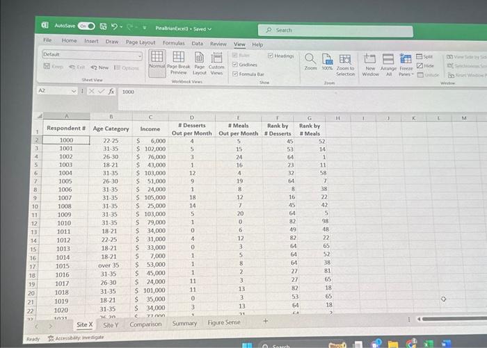
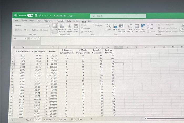
1. - On the Site X and Site Y worksheets, use the RANK.EQ function to rank each respondent by the number of desserts they eat out per month and the number of meals they eat out per month respectively (ranking from most desserts and meals out to the least).
2. - Freeze the top row on the Site X and Site Y worksheets to make the category headings visible at all times.
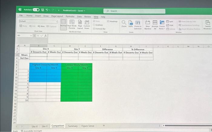
3. - In the Comparison worksheet, calculate the difference and percent difference of the mean and standard deviation for the data sets (Site X and Site Y) for the number of desserts and meals. Use the STDEV.S function for the standard deviation. The difference should be calculated as Site Y - Site X. The percent difference should be calculated as (Site Y - Site X) / Site X. Next, complete the table so that it lists the four highest number of desserts per month from each data set (Site X and Site Y) and the ten lowest number of meals eaten out by respondents for each of the data sets (Site X and Site Y).
4. - After looking at the data in the Comparison worksheet, you have decided that Site Y is the more attractive location for your new restaurant. On the Summary worksheet, use various formulas and functions to complete cells B1:B7 using only the data for Site Y.