please provide the excel equation with it

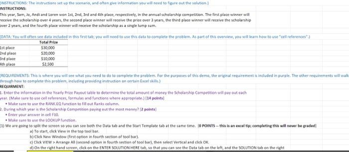
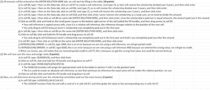
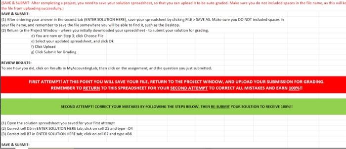
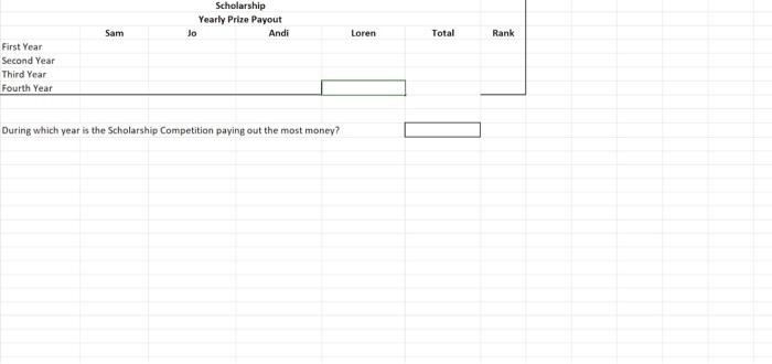
INSTRUCTIONS: The instructions set up the scenario, and often gleinformation you will need to figure out the solution INSTRUCTIONS: This year, Sam, Jo, Andi and Loren won 1st, 2nd, 3rd and 4th place, respectively, in the annual scholarship competition. The first place winner will receive the scholarship over 4 years, the second place winner will receive the prize over 3 years, the third place winner will receive the scholarship ver 2 years, and the fourth place winner will receive the scholarship as a single lumpsum. DATA: You will often see data included in this first tab; you will need to use this data to complete the problem. As part of this overview, you will learn how to use "celt retorences") Total Price 1st place $30,000 2nd place 520,000 3rd place 510,000 4th place $2.500 REQUIREMENTS: This is where you will see what you need to do to complete the problem. For the purpose of this demo, the original requirement is included in purple. The other requirements will walk through how to complete this problem, including providing instruction on certain Excel REQUIRMENT: Enter the information in the early Price Payout table to determine the total amount of money the Scholarship Competition will pay out each wear. (Make sure to use cell references, formulas and functions where appropriate.)114 points . Make sure to use the RANKEQ function to fill out Ranks column 2. During which year in the Scholarship Competition paying out the most money? 12 points) Enter your answer in cell 10. . Make sure to use the LOOKUP function 1) We are going to split the screen so you can see both the Data tab and the Start Template tab at the same time. TO POINTS - this is an excel tip: completing this will never be graded To start, click View in the top toolbar b) Click New Window first option in fourth section of toolbar), c) Click VEW> Arrange All (second option in fourth section of toolbar), then select Vertical and click OK On the right hand screen, click on the ENTER SOLUTION HERE tab, so that you can see the Data tab on the left, and the SOLUTION tab on the right (2) All answers will be entered on the ENTER SOLUTION HERE tab; we will start by filling in the table 10 points In cell 04, type then on the Data tab, click on cell 37 to create a cell reference; next type /4 as Sam will receive the scholarship divided over 4 years, and then click enter b) In cell C4, type then on the Data tab, click on cell 88, next type /3, as so will receive the scholarship divided over 3 years, and then dick enter In cell D4, type then on the Data tab, click on cell 09, next type /2, as Andi will receive the scholarship over 2 years, and then dick enter d) in cell 04.type = then on the Data tab, click on cell 810, and then click enter; Loren receives the scholarship as a lump sum, so no need to divide the amount e) In cell 05, type = then click on cell 04 on same tab (ENTER SOLUTION HERE), and then dick enter; since the scholarship is paid out in equal amounts, the amount paid out in the second Click on cell B5; click and hold on the small green square in the bottom right corner of the cell called the Sill handle), and then drag across to cell DS Your celt reference is copied across cells, since it is a relative cell reference, the reference changes relative to the position of the new cell You only drag ta cell Ds because Loren's scholarship was completely paid out in the first year a) In cell 16, type then click on cells on the same tab (ENTER SOLUTION HERE), and then click enter h) Click on cell 86, click and hold the fall handle and drag across to cell C6 . You only drag to cell C because Loren's scholarship was completely paid out in the first year and Andi's was completely paid out after the second in cel 87, type then click on cell B6 on the same tab (ENTER SOLUTION HERE), and then click enter DINTRODUCING ERRORS: In cells, type 5000; this is an error because we are not using a cell reference, we will get partial credit W) INTRODUCING ERRORS: In cell 07, types, this is an error because we are not using a cell reference AND because we entered the wrong values we will get no credit When we review, you will notice that we received partial credit in cell F, this is because we got the wrong final value, but used the correct formula (3) We will now sun the rows and assign ranka (4 points) a) In cell T4, type SUM[04 E4), and then click Enter 1) Click on cell 4click and hold the film handle and drag down to 7 In cell G4, type RANK COFF4,5$$4:$E$7,0) The RANKEQ function will assign the appropriate rank to the total incolumn with as the greatest total The Sicused to create an absolute cell reference, or one that continues to reference the exact same cel no matter the relative position; we use a) Click on cell 4, click and hold the fill handle and drag down to cell (4) Now, we will determine during which year the scholarship committee paid out the most money 12 points) a) In cell Flotype LOOKUP(1,6467,M4A7) The LOOKUP function finds the cell with a rank of 2 in cells 64:67, and then grabs the value in the corresponding row in cells A4:17 (SAVES SUBMIT After completing a project, you need to save your solution tradhet, so that you can upload it to be auto graded. Make sure you do not included spaces in the file name as this will be the file from uploading successfully SAVE & SUBMIT 11) After entering your answer in the second tab (ENTER SOLUTION HERE), save your spreadsheet by clicking FILE > SAVE AS. Make sure you DO NOT included spaces in your fle name, and remember to save the file somewhere you will be able to find such as the Desktop. (2) Return to the Project Window-where you initially downloaded your spreadsheet - to submit your solution for grading d) You are now on Step 3, click Choose File el Select your updated spreadsheet, and click OK 1) Click Upload a) Clide Sulimit for Grading REVIEW RESULTS: Yo see how you did, click on Results in MyAccountinya, then click on the assignment, and the question you just submitted. FIRST ATTEMPTI AT THIS POINT YOU WILL SAVE YOUR FILE, RETURN TO THE PROJECT WINDOW, AND UPLOAD YOUR SUBMISSION FOR GRADING REMEMBER TO RETURN TO THIS SPREADSHEET FOR YOUR SECOND ATTEMPT TO CORRECT ALL MISTAKES AND EARN 100%!! SECOND ATTEMPT CORRECT YOUR MISTAKES BY FOLLOWWG THE STEPS BELOW, THEN HE-SUBMIT YOUR SOULTION TO RECEIVE 100141 (1) Open the solution spreadsheet you saved for your first attempt (2) Correct cell OS in ENTER SOLUTION HERE tab, click on cells and type=D4 (3) Correct cell B7 in ENTER SOLUTION HERE tab; click on cell and type=B6 SAVE & SUBMIT Scholarship Yearly Prize Payout Jo Andi Sam Loren Total Rank First Year Second Year Third Year Fourth Year During which year is the Scholarship Competition paying out the most money? INSTRUCTIONS: The instructions set up the scenario, and often gleinformation you will need to figure out the solution INSTRUCTIONS: This year, Sam, Jo, Andi and Loren won 1st, 2nd, 3rd and 4th place, respectively, in the annual scholarship competition. The first place winner will receive the scholarship over 4 years, the second place winner will receive the prize over 3 years, the third place winner will receive the scholarship ver 2 years, and the fourth place winner will receive the scholarship as a single lumpsum. DATA: You will often see data included in this first tab; you will need to use this data to complete the problem. As part of this overview, you will learn how to use "celt retorences") Total Price 1st place $30,000 2nd place 520,000 3rd place 510,000 4th place $2.500 REQUIREMENTS: This is where you will see what you need to do to complete the problem. For the purpose of this demo, the original requirement is included in purple. The other requirements will walk through how to complete this problem, including providing instruction on certain Excel REQUIRMENT: Enter the information in the early Price Payout table to determine the total amount of money the Scholarship Competition will pay out each wear. (Make sure to use cell references, formulas and functions where appropriate.)114 points . Make sure to use the RANKEQ function to fill out Ranks column 2. During which year in the Scholarship Competition paying out the most money? 12 points) Enter your answer in cell 10. . Make sure to use the LOOKUP function 1) We are going to split the screen so you can see both the Data tab and the Start Template tab at the same time. TO POINTS - this is an excel tip: completing this will never be graded To start, click View in the top toolbar b) Click New Window first option in fourth section of toolbar), c) Click VEW> Arrange All (second option in fourth section of toolbar), then select Vertical and click OK On the right hand screen, click on the ENTER SOLUTION HERE tab, so that you can see the Data tab on the left, and the SOLUTION tab on the right (2) All answers will be entered on the ENTER SOLUTION HERE tab; we will start by filling in the table 10 points In cell 04, type then on the Data tab, click on cell 37 to create a cell reference; next type /4 as Sam will receive the scholarship divided over 4 years, and then click enter b) In cell C4, type then on the Data tab, click on cell 88, next type /3, as so will receive the scholarship divided over 3 years, and then dick enter In cell D4, type then on the Data tab, click on cell 09, next type /2, as Andi will receive the scholarship over 2 years, and then dick enter d) in cell 04.type = then on the Data tab, click on cell 810, and then click enter; Loren receives the scholarship as a lump sum, so no need to divide the amount e) In cell 05, type = then click on cell 04 on same tab (ENTER SOLUTION HERE), and then dick enter; since the scholarship is paid out in equal amounts, the amount paid out in the second Click on cell B5; click and hold on the small green square in the bottom right corner of the cell called the Sill handle), and then drag across to cell DS Your celt reference is copied across cells, since it is a relative cell reference, the reference changes relative to the position of the new cell You only drag ta cell Ds because Loren's scholarship was completely paid out in the first year a) In cell 16, type then click on cells on the same tab (ENTER SOLUTION HERE), and then click enter h) Click on cell 86, click and hold the fall handle and drag across to cell C6 . You only drag to cell C because Loren's scholarship was completely paid out in the first year and Andi's was completely paid out after the second in cel 87, type then click on cell B6 on the same tab (ENTER SOLUTION HERE), and then click enter DINTRODUCING ERRORS: In cells, type 5000; this is an error because we are not using a cell reference, we will get partial credit W) INTRODUCING ERRORS: In cell 07, types, this is an error because we are not using a cell reference AND because we entered the wrong values we will get no credit When we review, you will notice that we received partial credit in cell F, this is because we got the wrong final value, but used the correct formula (3) We will now sun the rows and assign ranka (4 points) a) In cell T4, type SUM[04 E4), and then click Enter 1) Click on cell 4click and hold the film handle and drag down to 7 In cell G4, type RANK COFF4,5$$4:$E$7,0) The RANKEQ function will assign the appropriate rank to the total incolumn with as the greatest total The Sicused to create an absolute cell reference, or one that continues to reference the exact same cel no matter the relative position; we use a) Click on cell 4, click and hold the fill handle and drag down to cell (4) Now, we will determine during which year the scholarship committee paid out the most money 12 points) a) In cell Flotype LOOKUP(1,6467,M4A7) The LOOKUP function finds the cell with a rank of 2 in cells 64:67, and then grabs the value in the corresponding row in cells A4:17 (SAVES SUBMIT After completing a project, you need to save your solution tradhet, so that you can upload it to be auto graded. Make sure you do not included spaces in the file name as this will be the file from uploading successfully SAVE & SUBMIT 11) After entering your answer in the second tab (ENTER SOLUTION HERE), save your spreadsheet by clicking FILE > SAVE AS. Make sure you DO NOT included spaces in your fle name, and remember to save the file somewhere you will be able to find such as the Desktop. (2) Return to the Project Window-where you initially downloaded your spreadsheet - to submit your solution for grading d) You are now on Step 3, click Choose File el Select your updated spreadsheet, and click OK 1) Click Upload a) Clide Sulimit for Grading REVIEW RESULTS: Yo see how you did, click on Results in MyAccountinya, then click on the assignment, and the question you just submitted. FIRST ATTEMPTI AT THIS POINT YOU WILL SAVE YOUR FILE, RETURN TO THE PROJECT WINDOW, AND UPLOAD YOUR SUBMISSION FOR GRADING REMEMBER TO RETURN TO THIS SPREADSHEET FOR YOUR SECOND ATTEMPT TO CORRECT ALL MISTAKES AND EARN 100%!! SECOND ATTEMPT CORRECT YOUR MISTAKES BY FOLLOWWG THE STEPS BELOW, THEN HE-SUBMIT YOUR SOULTION TO RECEIVE 100141 (1) Open the solution spreadsheet you saved for your first attempt (2) Correct cell OS in ENTER SOLUTION HERE tab, click on cells and type=D4 (3) Correct cell B7 in ENTER SOLUTION HERE tab; click on cell and type=B6 SAVE & SUBMIT Scholarship Yearly Prize Payout Jo Andi Sam Loren Total Rank First Year Second Year Third Year Fourth Year During which year is the Scholarship Competition paying out the most money