please put answer in solver. step by step directions. Thank you. will upvote.

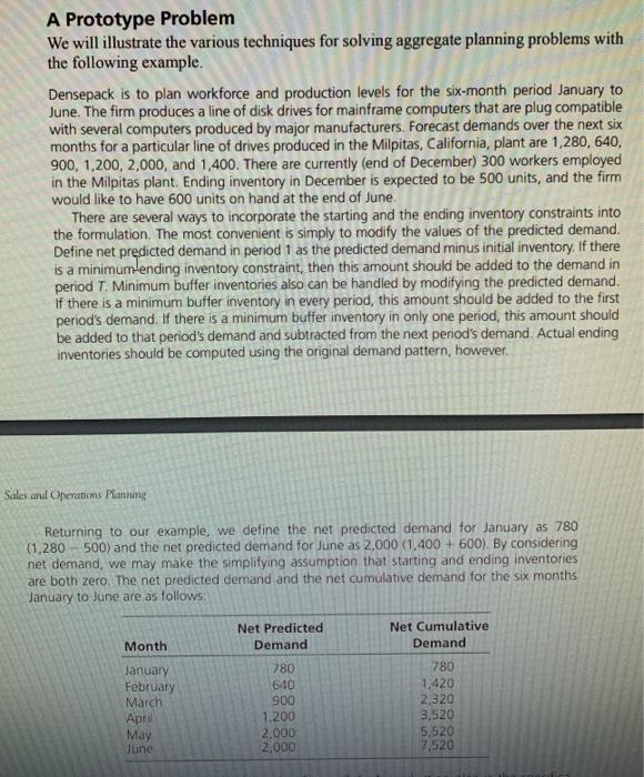
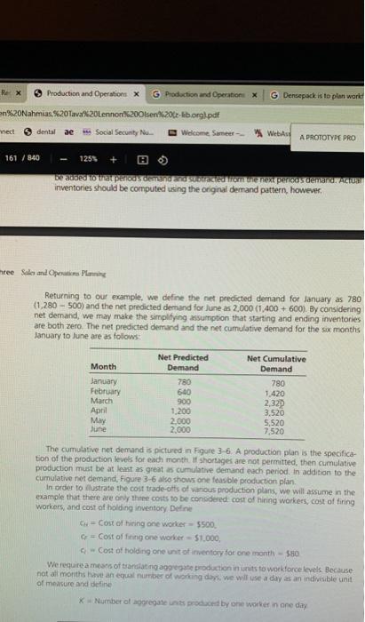
A Prototype Problem We will illustrate the various techniques for solving aggregate planning problems with the following example. Densepack is to plan workforce and production levels for the six-month period January to June. The firm produces a line of disk drives for mainframe computers that are plug compatible with several computers produced by major manufacturers. Forecast demands over the next six months for a particular line of drives produced in the Milpitas, California, plant are 1,280, 640, 900, 1,200, 2,000, and 1,400. There are currently (end of December) 300 workers employed in the Milpitas plant. Ending inventory in December is expected to be 500 units, and the firm would like to have 600 units on hand at the end of June. There are several ways to incorporate the starting and the ending inventory constraints into the formulation. The most convenient is simply to modify the values of the predicted demand. Define net predicted demand in period 1 as the predicted demand minus initial inventory. If there is a minimum ending inventory constraint, then this amount should be added to the demand in period T. Minimum buffer inventories also can be handled by modifying the predicted demand. If there is a minimum buffer inventory in every period, this amount should be added to the first period's demand. If there is a minimum buffer inventory in only one period, this amount should be added to that period's demand and subtracted from the next period's demand. Actual ending inventories should be computed using the original demand pattern, however. Sales and Operation Planning Returning to our example, we define the net predicted demand for January as 780 (1.280500) and the net predicted demand for June as 2,000 (1,400+600). By considering net demand, we may make the simplifying assumption that starting and ending inventories are both zero. The net predicted demand and the net cumulative demand for the six months January to June are as follows: Net Predicted Demand Net Cumulative Demand Month January February March April May June 780 640 900 1.200 2,000 2,000 780 1,420 2,320 3,520 5,520 7.520 Rex Production and Operations G Production and Operation X G Densepack is to plan world n%20Nahmias.%20Tava%20Lennon3.200lsen234t-lb.org.pdf Annect dental se Social Secunity Na Welcome Sameer - Webas A PROTOTYPE PRO 161/840 125 be able to perigosoene om en pericosdemar AIURE inventories should be computed using the original demand pattern, however, hree Sales and Operation Plan Returning to our example, we define the net predicted demand for January as 780 (1,280 - 500) and the net predicted demand for june as 2,000 (1,400 + 600). By considering net demand, we may make the simplifying assumption that starting and ending inventories are both zero. The net predicted demand and the net cumulative demand for the six months January to June are as folows: Month January February March April May June Net Predicted Demand 780 640 900 1.200 2.000 2,000 Net Cumulative Demand 780 1.420 2,320 3,520 5.520 7.520 The cumulative net demand is pictured in Figure 3-6. A production plan is the specifica tion of the production levels for each month. If shortages are not permitted, then cumulative production must be at least as great as cumulative demand each period. In addition to the cumulative net demand, Figure 3-6 also shows one feable production plan In order to flustrate the cost trade-offs of various production plans, we will assume in the example that there are only three costs to be considered cost of hiring workers, cost of firing workers, and cost of holding inventory Define Cost of hiring one worker 5500 Cost offing one worker = $1.000, Cost of holding one unit o inventory for one month - 580 We require a means of translating aggregate production in units to workforce levels Because not all months have an equal number of working days, we will use a day as an indivisible unit of measure and define Number of agregatets proded by one worker in one day A Prototype Problem We will illustrate the various techniques for solving aggregate planning problems with the following example. Densepack is to plan workforce and production levels for the six-month period January to June. The firm produces a line of disk drives for mainframe computers that are plug compatible with several computers produced by major manufacturers. Forecast demands over the next six months for a particular line of drives produced in the Milpitas, California, plant are 1,280, 640, 900, 1,200, 2,000, and 1,400. There are currently (end of December) 300 workers employed in the Milpitas plant. Ending inventory in December is expected to be 500 units, and the firm would like to have 600 units on hand at the end of June. There are several ways to incorporate the starting and the ending inventory constraints into the formulation. The most convenient is simply to modify the values of the predicted demand. Define net predicted demand in period 1 as the predicted demand minus initial inventory. If there is a minimum ending inventory constraint, then this amount should be added to the demand in period T. Minimum buffer inventories also can be handled by modifying the predicted demand. If there is a minimum buffer inventory in every period, this amount should be added to the first period's demand. If there is a minimum buffer inventory in only one period, this amount should be added to that period's demand and subtracted from the next period's demand. Actual ending inventories should be computed using the original demand pattern, however. Sales and Operation Planning Returning to our example, we define the net predicted demand for January as 780 (1.280500) and the net predicted demand for June as 2,000 (1,400+600). By considering net demand, we may make the simplifying assumption that starting and ending inventories are both zero. The net predicted demand and the net cumulative demand for the six months January to June are as follows: Net Predicted Demand Net Cumulative Demand Month January February March April May June 780 640 900 1.200 2,000 2,000 780 1,420 2,320 3,520 5,520 7.520 Rex Production and Operations G Production and Operation X G Densepack is to plan world n%20Nahmias.%20Tava%20Lennon3.200lsen234t-lb.org.pdf Annect dental se Social Secunity Na Welcome Sameer - Webas A PROTOTYPE PRO 161/840 125 be able to perigosoene om en pericosdemar AIURE inventories should be computed using the original demand pattern, however, hree Sales and Operation Plan Returning to our example, we define the net predicted demand for January as 780 (1,280 - 500) and the net predicted demand for june as 2,000 (1,400 + 600). By considering net demand, we may make the simplifying assumption that starting and ending inventories are both zero. The net predicted demand and the net cumulative demand for the six months January to June are as folows: Month January February March April May June Net Predicted Demand 780 640 900 1.200 2.000 2,000 Net Cumulative Demand 780 1.420 2,320 3,520 5.520 7.520 The cumulative net demand is pictured in Figure 3-6. A production plan is the specifica tion of the production levels for each month. If shortages are not permitted, then cumulative production must be at least as great as cumulative demand each period. In addition to the cumulative net demand, Figure 3-6 also shows one feable production plan In order to flustrate the cost trade-offs of various production plans, we will assume in the example that there are only three costs to be considered cost of hiring workers, cost of firing workers, and cost of holding inventory Define Cost of hiring one worker 5500 Cost offing one worker = $1.000, Cost of holding one unit o inventory for one month - 580 We require a means of translating aggregate production in units to workforce levels Because not all months have an equal number of working days, we will use a day as an indivisible unit of measure and define Number of agregatets proded by one worker in one day