Please reference the photos in order and solve them: Date formats that begin with an asterisk $(*)$ will always display the correct regional date format.

This is recommended when sharing a file internationally.

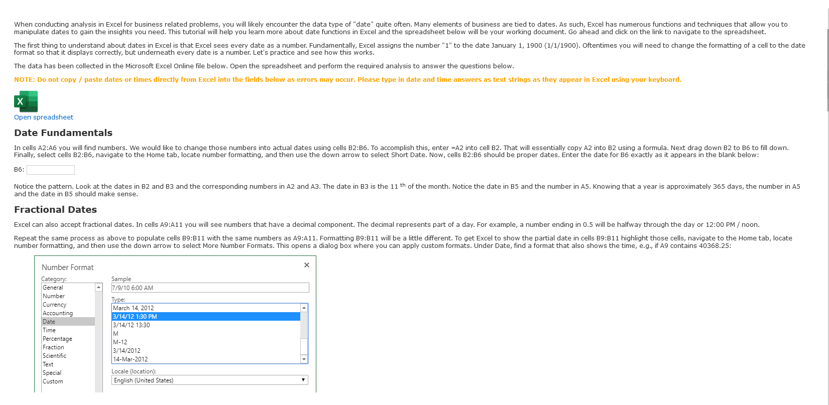
Cells B$9$:B$11$ should now show the date and partial date as time of day. Enter the values shown in cells B$9$:B$11$ exactly as they appear in the blanks below:

B$9$:

B$10$:

B$11$:

Built in Excel Functions

Two Excel date functions that are good to know are TODAY$()$ and NOW$().$ In cells E$2$ and E$3$ practice those two functions. Three important points about TODAY$()$ and NOW$().$

$1.$ They do not take arguments; just open and closed parenthesis $().$ running Excel. That could be on your laptop or in the case of the cloud, halfway around the world. So just be mindful.

Targeted Date Functions

Date Parts

E$7$:

E$8$:

E$9$:

Useful relative dates Useful relative dates

Many deadlines in business are at the end of the month. Therefore, Excel has a function called EOMONTH that can help you find that automatically. Help with EOMONTH can be found at this link. To find the end of the month for the date in E$6,$ in E$11$ insert $=$EOMONTH$($E$6,0).$ The zero tells Excel to stay in the month specified in the E$6$ date. Enter the value in E$11$ below exactly as it appears:

E$11$: to obtain the beginning of the month. You just need to add one more day to $\backslash (=\backslash )$ EOMONTH $(\backslash (\backslash$mathrm$\{$E$\}6,-1\backslash )).$ Since Excel sees dates and numbers, just $+1.$

E$12$:

E$13$: four months. That would take us to the end of the previous year. Then add one day to get to the beginning of the current year.

Using EOMONTH, E$6,$ E$8,$ and $+1,$ in cell E$14$ find the first day of the year for the date shown in E$6.$

E$14$: days that have occurred between the beginning of the year date $($which you already found$)$ and the date in E$6.$ Enter the result of your I$3$ calculation below:

I$3$: problem use a basis of $1.$ More help with YEARFRAC can be found at this link. have the result show as a percentage, you may need to format the cell as a percent.

In cell I$4,$ find the faction of the year represented between the date in E$6$ and the beginning of the year $($to $1$ decimal$).$ Enter the percentage below without the $\backslash \%$ sign.

I$4$:

$\backslash \%$

In cell I$5,$ find the fraction of the year represented between the date in E$6$ and the beginning of the month $($to $1$ decimal$).$ Enter the percentage below without the $\backslash \%$ sign.

link. WEEKDAY function inside the TEXT function. WEEKDAY function inside the TEXT function. formatting instruction to the TEXT function. Enter the day of the week from I$7$ below $($capitalize the first letter$).$

$17$: $\backslash (=\backslash )$ TEXT$($date$,"$mmmm$").$ Enter the month name from I$10$ below $($capitalize the first letter$).$

I$10$: beginning of the month and end of month in column E and place the result in I$12.$ How many workdays are in the current month? Ignore any holidays and leave the "Holidays" argument blank.

I$12$: of workdays you specify have happened? Help with WORKDAY function can be found at this link.

Data Table use the techniques you learned above to populate each row with the month and day of the week based on the date in column A $.$

Revenue Pivot Table

What is the lowest sum of revenue in the pivot table? $($Note: Conditional formatting can help!$)$

What is the highest sum of revenue in the pivot table? $($Note: Conditional formatting can help!$)$ I$12$: of workdays you specify have happened? Help with WORKDAY function can be found at this link. use the WORKDAY function to find the date that is $30$ workdays from the date in E$6.$ Ignore any holidays and leave the "Holidays" argument blank.

I$13$:

I$14$:

Data Table use the techniques you learned above to populate each row with the month and day of the week based on the date in column A$.$

Revenue Pivot Table

What is the lowest sum of revenue in the pivot table? $($Note: Conditional formatting can help!$)$

$-$ Lowest revenue Month Day

What is the highest sum of revenue in the pivot table? $($Note: Conditional formatting can help!$)$

Highest revenue

Month Day

$\backslash$$

Target Pivot Table second time in the Values field of the pivot table.

Which month hit the target revenue most frequently?

Month: