Please show all steps and formulas. i'm using office 360.

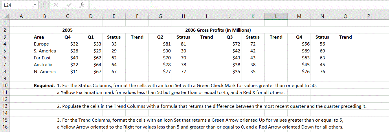
L24 B D E F G H 1 K M N 0 P 1 2 Trend Trend Trend 3 4 Status 56 5 6 7 Area Europe S. America Far East Australia N. America 2005 Q4 $32 $26 $49 $22 $11 Q1 $33 $29 $62 $64 $67 Status 33 29 62 64 67 Q2 $81 $30 $70 $78 $77 2006 Gross Profits (in Millions) Status Trend Q3 Status 81 $72 72 30 $42 42 70 $43 43 78 $38 38 77 $35 35 Q4 $56 $69 $63 $45 $76 69 63 45 76 8 9 Required: 1. For the Status Columns, format the cells with an Icon Set with a Green Check Mark for values greater than or equal to 50, a Yellow Exclamation mark for values less than 50 but greater than or equal to 45, and a Red X for all others. 10 11 12 13 14 15 16 2. Populate the cells in the Trend Columns with a formula that returns the difference between the most recent quarter and the quarter preceding it. 3. For the Trend Columns, format the cells with an Icon Set that returns a Green Arrow oriented Up for values greater than or equal to 5, a Yellow Arrow oriented to the Right for values less than 5 and greater than or equal to 0, and a Red Arrow oriented Down for all others