please show the formulas on the excel sheet

Thats all the information provided. please show formulas on the excel sheet

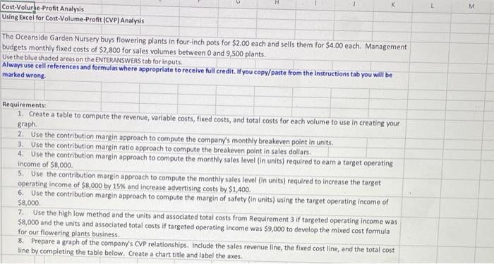
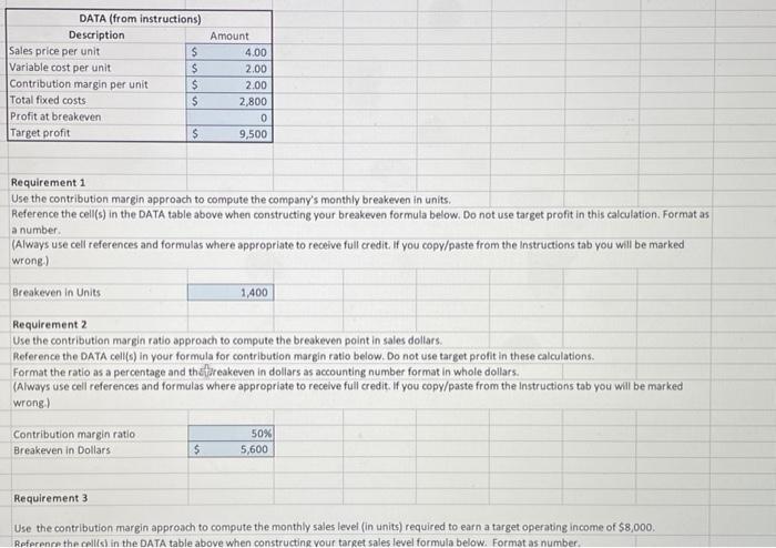
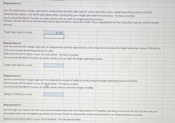
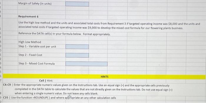
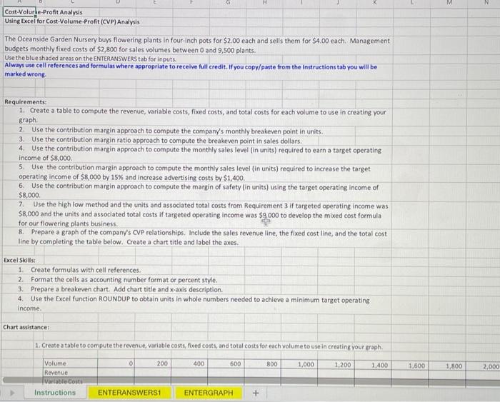
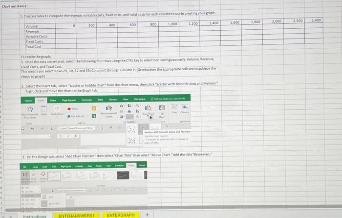
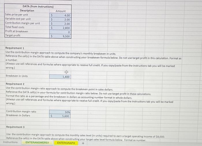
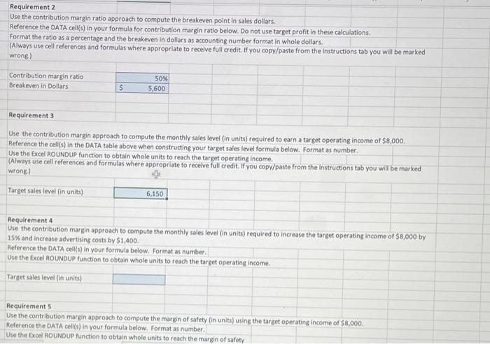
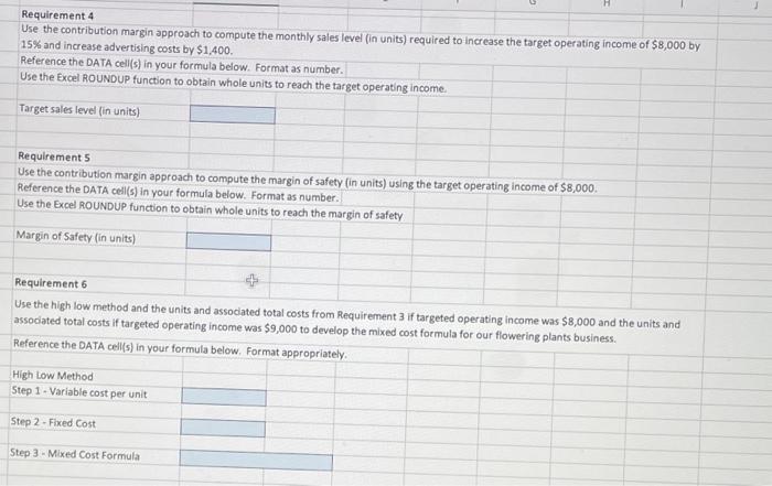
The Oceanside Garden Nursery buys flowering plants in four-inch pots for $2.00 each and sells them for $4.00 each. Management budgets monthly fixed costs of $2,800 for sales volumes between 0 and 9,500 plants. Use the blue shaded areas on the ENTERANSWEAS tab for inputs. Always use cell references and formulas where appropriate to receive full credit. If you copy/paste from the instructions tab you will be marked wrong. Requirements: 1. Create a table to compute the revenue, variable costs, fixed costs, and total costs for each volume to use in creating your graph. 2. Use the contribution margin approach to compute the company's monthly breakeven point in units. 3. Use the contribution margin ratio approach to compute the breakeven point in sales dollars. 4. Use the contribution margin approach to compute the monthly sales level (in units) required to earn a target operating income of $8,000. 5. Use the contribution margin approach to compute the monthly sales level (in units) required to increase the target operating income of $8,000 by 15% and increase advertising costs by $1,400. 6. Use the contribution margin approach to compute the margin of safety (in units) using the target operating income of 58,000 . 7. Use the high low method and the units and associated total costs from Requirement 3 if targeted operating income was $8,000 and the units and associated total costs if targeted operating income was $9,000 to develop the mixed cost formula for our flowering plants business. 8. Prepare a graph of the company's CVP relationships. Include the sales revenue line, the fixed cost line, and the total cost line by completing the table below. Create a chart title and label the axes. Use the contribution margin approach to compute the company's monthly breakeven in units. Reference the cell(s) in the DATA table above when constructing your breakeven formula below. Do not use target profit in this calculation. Format as a number. (Always use cell references and formulas where appropriate to receive full credit. If you copy/paste from the Instructions tab you will be marked wrong.) Breakeven in Units 1,400 Requirement 2 Use the contribution margin ratio approach to compute the breakeven point in sales dollars. Reference the DATA cell(s) in your formula for contribution margin ratio below. Do not use target profit in these calculations. Format the ratio as a percentage and thstis eakeven in dollars as accounting number format in whole dollars. (Always use cell references and formulas where appropriate to receive full credit. If you copy/paste from the Instructions tab you will be marked Wrong) Requirement 3 Use the contribution margin approach to compute the monthly sales level (in units) required to earn a target operating income of $8,000. Referenre the rell(s) in the DATA table above when constructing vour target sales level formula below. Format as number. Requirement 3 Use the contribution margin approach to compute the monthly sales level (in units) required to earn a target operating income of $8,000. Reference the cell(s) in the DATA table above when constructing your target sales level formula below. Format as number. Use the Excel ROUNDUP function to obtain whole units to reach the target operating income. (Always use cell references and formulas where appropriate to recelve full credit. If you copy/paste from the Instructions tab you will be marked wrong.) Requirement 4 Use the contribution margin approach to compute the monthly sales level (in units) required to increase the target operating income of $8,000 by 15% and increase advertising costs by $1,400. Reference the DATA cell(s) in your formula below. Format as number. Use the Excel ROUNDUP function to obtain whole units to reach the target operating income. Target sales level (in units) Requirement 5 Use the contribution margin approach to compute the margin of safety (in units) using the target operating income of $8,000. Reference the DATA cell(s) in your formyla below. Format as number. Use the Excel ROUNDUP function to obtain whole units to reach the margin of safety Margin of Safety (in units) Requirement 6 Use the high low method and the units and associated total costs from Requirement 3 if targeted operating income was $8,000 and the units and associated total costs if targeted operating income was $9,000 to develop the mixed cost formula for our flowering plants business. Reference the DATA cell(s) in your formula below. Format appropriately. Requirement 6 Use the high low method and the units and associated total costs from Requirement 3 if targeted operating income was $8,000 and the units and associated total costs if targeted operating income was $9,000 to develop the mixed cost formula for our flowering plants business. Reference the DATA cell(s) in your formula below. Format appropriately. C4:C9 | Enter the appropriate numeric values given on the Instructions tab. Use an equal sign ( ) and the appropriate cells previously completed in the DATA table to calculate the values that are not directly given on the Instructions tab. Do not use equal sign (=) when entering a single numeric value. Do not leave any cells blank. C35 | Use the function =ROUNDUP() and where appifopriate an any other calculation cells The Oceanside Garden Nursery bioys flowering plants in four-inch pots for $2,00 each and sells them for $4,00 each. Management budgets monthly fixed costs of $2,800 for sales volumes between 0 and 9,500 plants. Use the blue shaded areas on the ENTERANSWERS tab for inputs. Always use cell references and formulas where appropriate to receive full credit. If you copy/paste from the instructions tab you will be marked wrong. Requirements: 1. Create a table to compute the revenue, variable costs, fixed costs, and total costs for each volume to use in creating your graph. 2. Use the contribution margin approach to compute the company's monthly breakeven point in units. 3. Use the contribution margin ratio approach to compute the breakeven point in sales dollars. 4. Use the contribution margin approach to compute the monthly sales level (in units) required to earn a target operating income of $8,000. 5. Use the contribution margin approach to compute the monthly sales level (in units) required to increase the target operating income of $8,000 by 15% and increase advertising costs by $1,400. 6. Use the contribution margin approach to compute the margin of safety (in units) using the target operating income of $8,000. 7. Use the high low method and the units and associated total costs from Requirement 3 if targeted operating income was $8,000 and the units and associated total costs if targeted operating income was $9,000 to develop the mixed cost formula for our flowering plants business. 8. Prepare a graph of the company's CVP relationships. Include the sales revenue line, the fixed cost line, and the total cost line by completing the table below. Create a chart title and label the axes. Excelskilts: 1. Create formulas with cell references. 2. Format the cells as accounting number format or percent style. 3. Prepare a breakeven chart. Add chart title and x-axis description. 4. Use the Excel function ROUNDUP to obtain units in whole numbers needed to achleve a minimum target operating income. Chart assistance: 1. Create a table to compute the revenue, variable costs, fixed costi, and total costs for each volume to use in creating your graph. 1. Once the data are entered, ueect the following four rowi using the Crimt kery to select rionsentiguous celli volume, Revenum, fixed Costh, and Tetal Cont. This means you wect Rows 29,30,32 ard 33, Column C through Column Pi ior whatever the appropriate cells are to achicve the fectsted maphy 2. Select the lesert tab, weet "zatter or bubble chart" from the chart ment, then click "Seatter with Senooth Lines and Maskers:" Night cliek and move the chart to the Graph tab 1. Dn the Design tab, select "Add Chart Demert" then select "Chart Title" then yelect "Above Chart. "Add the title "3reakeven: Requirement 1 Use the contribution margin approach to compute the company's monthly breakeven in units. Reference the cell(s) in the DATA table above when constructing your breakeven formula below. Do not use target profit in this calculation. Format as a number. (Always use cell references and formulas where appropriate to receive full credit. If you copy/paste from the lnstructions tab you will be marked wrong.) Use the contribution margin ratio approach to compute the breakeven point in sales dollars. Reference the DATA cell(s) in your formula for contribution margin ratio below. Do not use target profit in these calculations. Format the ratio as a percentage and the breakeven in dollars as accounting number format in whole dollars. (Always use cell references and formulas where appropriate to receive full credit. If you copy/paste from the Instructions tab you will be marked wrong.) Requirement 3 Use the contribution margin approach to compute the monthly sales level (in units) required to earn a target operating income of $8,000. Reference the cell(s) in the DATA table above when constructing your target sales level formula below. Format as number. Use the contribution margin ratio approach to compute the breakeven point in sales dollars. Reference the DATA cell(s) in your formula for contribution margin ratio below. Do not use target profit in these calculations. Format the ratio as a percentage and the breakeven in dollars as accounting number format in whole dollars. (Always use cell references and formulas where appropriate to receive full credit. If you copy/paste from the instructions tab you will be marked wrong.) Requirement 3 Use the contribution margin approach to compute the monthly sales level (in units) required to earn a target operating income of $8,000. Reference the cell(s) in the DATA table above when constructing your target sales level formula below. Format as number. Use the Excel ROUNDUP function to obtain whole units to reach the target operating income. (Always use cell references and formulas where appropriate to receive full credit. If you copy/paste from the instructions tab you will be marked wrong.) Requirement 4 Use the contribution margin approach to compute the monthly sales level (in units) required to increase the target operating income of $8,000 by 15% and increase advertising costs by $1,400. Aeference the DATA cell(s) in your formula below. Format as number. Use the Excel hOUNDUP function to obtain whole units to reach the target operating income. Target sales level (in units) Requirement 5 Use the contribution margin approach to compute the margin of safety (in units) using the target operating income of $8,000. Reference the DATA cell(s) in your formula below. Format as number. Use the Excel HOUNDUP function to obtain whole units to reach the margin of safety Requirement 4 Use the contribution margin approach to compute the monthly sales level (in units) required to increase the target operating income of $8,000 by 15% and increase advertising costs by $1,400. Reference the DATA cell(s) in your formula below. Format as number. Use the Excel ROUNDUP function to obtain whole units to reach the target operating income. Target sales level (in units) Requirement 5 Use the contribution margin approach to compute the margin of safety (in units) using the target operating income of $8,000. Reference the DATA cell(s) in your formula below. Format as number. Use the Excel ROUNDUP function to obtain whole units to reach the margin of safety Margin of Safety Use the high low method and the units and associated total costs from Requirement 3 if targeted operating income was $8,000 and the units and associated total costs if targeted operating income was $9,000 to develop the mixed cost formula for our flowering plants business. Reference the DATA cell(s) in your formula below. Format appropriately. High Low Method Step 1-Variable cost per unit Step 2-Fixed Cost Step-3 - Mixed Cost Formula The Oceanside Garden Nursery buys flowering plants in four-inch pots for $2.00 each and sells them for $4.00 each. Management budgets monthly fixed costs of $2,800 for sales volumes between 0 and 9,500 plants. Use the blue shaded areas on the ENTERANSWEAS tab for inputs. Always use cell references and formulas where appropriate to receive full credit. If you copy/paste from the instructions tab you will be marked wrong. Requirements: 1. Create a table to compute the revenue, variable costs, fixed costs, and total costs for each volume to use in creating your graph. 2. Use the contribution margin approach to compute the company's monthly breakeven point in units. 3. Use the contribution margin ratio approach to compute the breakeven point in sales dollars. 4. Use the contribution margin approach to compute the monthly sales level (in units) required to earn a target operating income of $8,000. 5. Use the contribution margin approach to compute the monthly sales level (in units) required to increase the target operating income of $8,000 by 15% and increase advertising costs by $1,400. 6. Use the contribution margin approach to compute the margin of safety (in units) using the target operating income of 58,000 . 7. Use the high low method and the units and associated total costs from Requirement 3 if targeted operating income was $8,000 and the units and associated total costs if targeted operating income was $9,000 to develop the mixed cost formula for our flowering plants business. 8. Prepare a graph of the company's CVP relationships. Include the sales revenue line, the fixed cost line, and the total cost line by completing the table below. Create a chart title and label the axes. Use the contribution margin approach to compute the company's monthly breakeven in units. Reference the cell(s) in the DATA table above when constructing your breakeven formula below. Do not use target profit in this calculation. Format as a number. (Always use cell references and formulas where appropriate to receive full credit. If you copy/paste from the Instructions tab you will be marked wrong.) Breakeven in Units 1,400 Requirement 2 Use the contribution margin ratio approach to compute the breakeven point in sales dollars. Reference the DATA cell(s) in your formula for contribution margin ratio below. Do not use target profit in these calculations. Format the ratio as a percentage and thstis eakeven in dollars as accounting number format in whole dollars. (Always use cell references and formulas where appropriate to receive full credit. If you copy/paste from the Instructions tab you will be marked Wrong) Requirement 3 Use the contribution margin approach to compute the monthly sales level (in units) required to earn a target operating income of $8,000. Referenre the rell(s) in the DATA table above when constructing vour target sales level formula below. Format as number. Requirement 3 Use the contribution margin approach to compute the monthly sales level (in units) required to earn a target operating income of $8,000. Reference the cell(s) in the DATA table above when constructing your target sales level formula below. Format as number. Use the Excel ROUNDUP function to obtain whole units to reach the target operating income. (Always use cell references and formulas where appropriate to recelve full credit. If you copy/paste from the Instructions tab you will be marked wrong.) Requirement 4 Use the contribution margin approach to compute the monthly sales level (in units) required to increase the target operating income of $8,000 by 15% and increase advertising costs by $1,400. Reference the DATA cell(s) in your formula below. Format as number. Use the Excel ROUNDUP function to obtain whole units to reach the target operating income. Target sales level (in units) Requirement 5 Use the contribution margin approach to compute the margin of safety (in units) using the target operating income of $8,000. Reference the DATA cell(s) in your formyla below. Format as number. Use the Excel ROUNDUP function to obtain whole units to reach the margin of safety Margin of Safety (in units) Requirement 6 Use the high low method and the units and associated total costs from Requirement 3 if targeted operating income was $8,000 and the units and associated total costs if targeted operating income was $9,000 to develop the mixed cost formula for our flowering plants business. Reference the DATA cell(s) in your formula below. Format appropriately. Requirement 6 Use the high low method and the units and associated total costs from Requirement 3 if targeted operating income was $8,000 and the units and associated total costs if targeted operating income was $9,000 to develop the mixed cost formula for our flowering plants business. Reference the DATA cell(s) in your formula below. Format appropriately. C4:C9 | Enter the appropriate numeric values given on the Instructions tab. Use an equal sign ( ) and the appropriate cells previously completed in the DATA table to calculate the values that are not directly given on the Instructions tab. Do not use equal sign (=) when entering a single numeric value. Do not leave any cells blank. C35 | Use the function =ROUNDUP() and where appifopriate an any other calculation cells The Oceanside Garden Nursery bioys flowering plants in four-inch pots for $2,00 each and sells them for $4,00 each. Management budgets monthly fixed costs of $2,800 for sales volumes between 0 and 9,500 plants. Use the blue shaded areas on the ENTERANSWERS tab for inputs. Always use cell references and formulas where appropriate to receive full credit. If you copy/paste from the instructions tab you will be marked wrong. Requirements: 1. Create a table to compute the revenue, variable costs, fixed costs, and total costs for each volume to use in creating your graph. 2. Use the contribution margin approach to compute the company's monthly breakeven point in units. 3. Use the contribution margin ratio approach to compute the breakeven point in sales dollars. 4. Use the contribution margin approach to compute the monthly sales level (in units) required to earn a target operating income of $8,000. 5. Use the contribution margin approach to compute the monthly sales level (in units) required to increase the target operating income of $8,000 by 15% and increase advertising costs by $1,400. 6. Use the contribution margin approach to compute the margin of safety (in units) using the target operating income of $8,000. 7. Use the high low method and the units and associated total costs from Requirement 3 if targeted operating income was $8,000 and the units and associated total costs if targeted operating income was $9,000 to develop the mixed cost formula for our flowering plants business. 8. Prepare a graph of the company's CVP relationships. Include the sales revenue line, the fixed cost line, and the total cost line by completing the table below. Create a chart title and label the axes. Excelskilts: 1. Create formulas with cell references. 2. Format the cells as accounting number format or percent style. 3. Prepare a breakeven chart. Add chart title and x-axis description. 4. Use the Excel function ROUNDUP to obtain units in whole numbers needed to achleve a minimum target operating income. Chart assistance: 1. Create a table to compute the revenue, variable costs, fixed costi, and total costs for each volume to use in creating your graph. 1. Once the data are entered, ueect the following four rowi using the Crimt kery to select rionsentiguous celli volume, Revenum, fixed Costh, and Tetal Cont. This means you wect Rows 29,30,32 ard 33, Column C through Column Pi ior whatever the appropriate cells are to achicve the fectsted maphy 2. Select the lesert tab, weet "zatter or bubble chart" from the chart ment, then click "Seatter with Senooth Lines and Maskers:" Night cliek and move the chart to the Graph tab 1. Dn the Design tab, select "Add Chart Demert" then select "Chart Title" then yelect "Above Chart. "Add the title "3reakeven: Requirement 1 Use the contribution margin approach to compute the company's monthly breakeven in units. Reference the cell(s) in the DATA table above when constructing your breakeven formula below. Do not use target profit in this calculation. Format as a number. (Always use cell references and formulas where appropriate to receive full credit. If you copy/paste from the lnstructions tab you will be marked wrong.) Use the contribution margin ratio approach to compute the breakeven point in sales dollars. Reference the DATA cell(s) in your formula for contribution margin ratio below. Do not use target profit in these calculations. Format the ratio as a percentage and the breakeven in dollars as accounting number format in whole dollars. (Always use cell references and formulas where appropriate to receive full credit. If you copy/paste from the Instructions tab you will be marked wrong.) Requirement 3 Use the contribution margin approach to compute the monthly sales level (in units) required to earn a target operating income of $8,000. Reference the cell(s) in the DATA table above when constructing your target sales level formula below. Format as number. Use the contribution margin ratio approach to compute the breakeven point in sales dollars. Reference the DATA cell(s) in your formula for contribution margin ratio below. Do not use target profit in these calculations. Format the ratio as a percentage and the breakeven in dollars as accounting number format in whole dollars. (Always use cell references and formulas where appropriate to receive full credit. If you copy/paste from the instructions tab you will be marked wrong.) Requirement 3 Use the contribution margin approach to compute the monthly sales level (in units) required to earn a target operating income of $8,000. Reference the cell(s) in the DATA table above when constructing your target sales level formula below. Format as number. Use the Excel ROUNDUP function to obtain whole units to reach the target operating income. (Always use cell references and formulas where appropriate to receive full credit. If you copy/paste from the instructions tab you will be marked wrong.) Requirement 4 Use the contribution margin approach to compute the monthly sales level (in units) required to increase the target operating income of $8,000 by 15% and increase advertising costs by $1,400. Aeference the DATA cell(s) in your formula below. Format as number. Use the Excel hOUNDUP function to obtain whole units to reach the target operating income. Target sales level (in units) Requirement 5 Use the contribution margin approach to compute the margin of safety (in units) using the target operating income of $8,000. Reference the DATA cell(s) in your formula below. Format as number. Use the Excel HOUNDUP function to obtain whole units to reach the margin of safety Requirement 4 Use the contribution margin approach to compute the monthly sales level (in units) required to increase the target operating income of $8,000 by 15% and increase advertising costs by $1,400. Reference the DATA cell(s) in your formula below. Format as number. Use the Excel ROUNDUP function to obtain whole units to reach the target operating income. Target sales level (in units) Requirement 5 Use the contribution margin approach to compute the margin of safety (in units) using the target operating income of $8,000. Reference the DATA cell(s) in your formula below. Format as number. Use the Excel ROUNDUP function to obtain whole units to reach the margin of safety Margin of Safety Use the high low method and the units and associated total costs from Requirement 3 if targeted operating income was $8,000 and the units and associated total costs if targeted operating income was $9,000 to develop the mixed cost formula for our flowering plants business. Reference the DATA cell(s) in your formula below. Format appropriately. High Low Method Step 1-Variable cost per unit Step 2-Fixed Cost Step-3 - Mixed Cost Formula