please solve question 2

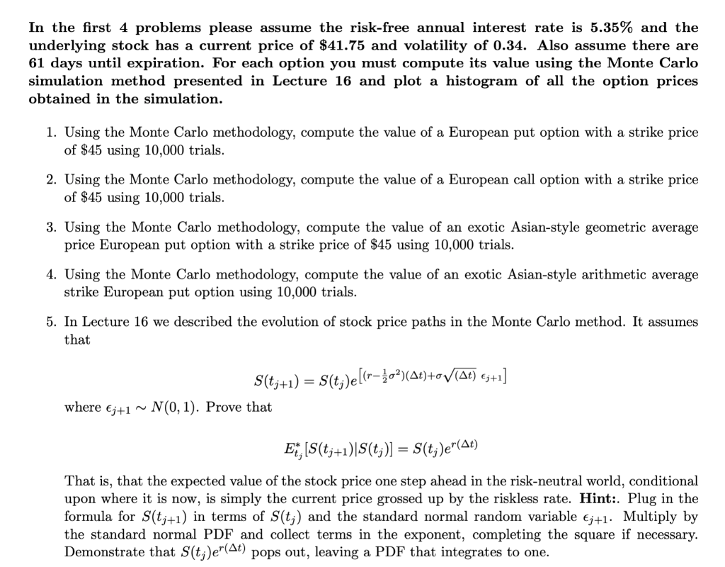
In the first 4 problems please assume the risk-free annual interest rate is 5.35% and the underlying stock has a current price of $41.75 and volatility of 0.34. Also assume there are 61 days until expiration. For each option you must compute its value using the Monte Carlo simulation method presented in Lecture 16 and plot a histogram of all the option prices obtained in the simulation. 1. Using the Monte Carlo methodology, compute the value of a European put option with a strike price of $45 using 10,000 trials. 2. Using the Monte Carlo methodology, compute the value of a European call option with a strike price of $45 using 10,000 trials. 3. Using the Monte Carlo methodology, compute the value of an exotic Asian-style geometric average price European put option with a strike price of $45 using 10,000 trials. 4. Using the Monte Carlo methodology, compute the value of an exotic Asian-style arithmetic average strike European put option using 10,000 trials. 5. In Lecture 16 we described the evolution of stock price paths in the Monte Carlo method. It assumes that S(tj+1) = S(t;)e[(r=o?)(41)+oV(At) 3+1] N(0,1). Prove that where j+1 ~ Et, [S(tj+1)|S(t;)] = S(tj)e"(At) That is, that the expected value of the stock price one step ahead in the risk-neutral world, conditional upon where it is now, is simply the current price grossed up by the riskless rate. Hint:. Plug in the formula for S(tj+1) in terms of S(tj) and the standard normal random variable 3+1. Multiply by the standard normal PDF and collect terms in the exponent, completing the square if necessary. Demonstrate that S(tj)er(At) pops out, leaving a PDF that integrates to one. In the first 4 problems please assume the risk-free annual interest rate is 5.35% and the underlying stock has a current price of $41.75 and volatility of 0.34. Also assume there are 61 days until expiration. For each option you must compute its value using the Monte Carlo simulation method presented in Lecture 16 and plot a histogram of all the option prices obtained in the simulation. 1. Using the Monte Carlo methodology, compute the value of a European put option with a strike price of $45 using 10,000 trials. 2. Using the Monte Carlo methodology, compute the value of a European call option with a strike price of $45 using 10,000 trials. 3. Using the Monte Carlo methodology, compute the value of an exotic Asian-style geometric average price European put option with a strike price of $45 using 10,000 trials. 4. Using the Monte Carlo methodology, compute the value of an exotic Asian-style arithmetic average strike European put option using 10,000 trials. 5. In Lecture 16 we described the evolution of stock price paths in the Monte Carlo method. It assumes that S(tj+1) = S(t;)e[(r=o?)(41)+oV(At) 3+1] N(0,1). Prove that where j+1 ~ Et, [S(tj+1)|S(t;)] = S(tj)e"(At) That is, that the expected value of the stock price one step ahead in the risk-neutral world, conditional upon where it is now, is simply the current price grossed up by the riskless rate. Hint:. Plug in the formula for S(tj+1) in terms of S(tj) and the standard normal random variable 3+1. Multiply by the standard normal PDF and collect terms in the exponent, completing the square if necessary. Demonstrate that S(tj)er(At) pops out, leaving a PDF that integrates to one