Please solve the following Time Series problem using R Studio and share the necessary plots, graphs and source codes.

data set -> austres -> data() -> built-in data set in R Studio

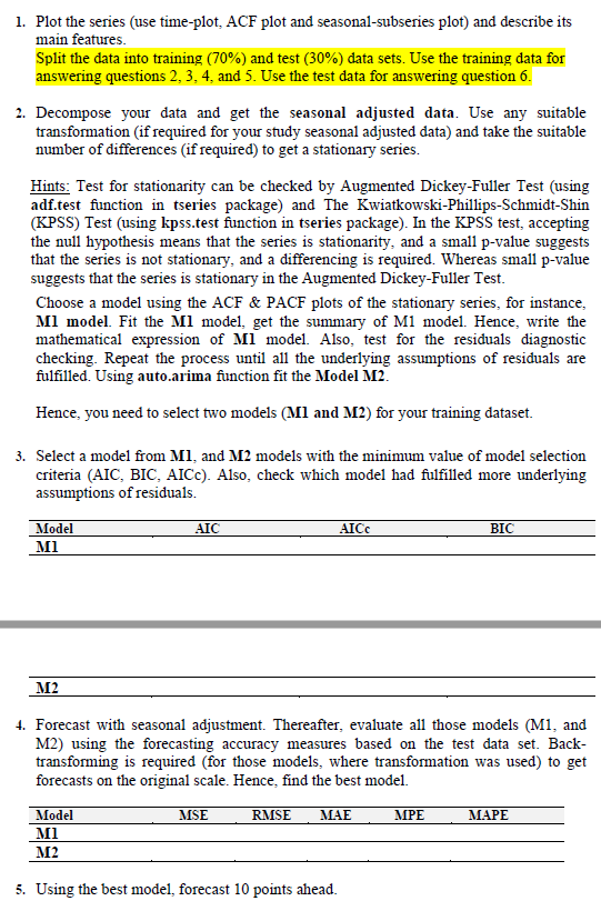
1. Plot the series (use time-plot, ACF plot and seasonal-subseries plot) and describe its main features. Split the data into training (70\%) and test (30%) data sets. Use the training data for answering questions 2,3,4, and 5. Use the test data for answering question 6 . 2. Decompose your data and get the seasonal adjusted data. Use any suitable transformation (if required for your study seasonal adjusted data) and take the suitable number of differences (if required) to get a stationary series. Hints: Test for stationarity can be checked by Augmented Dickey-Fuller Test (using adf.test function in tseries package) and The Kwiatkowski-Phillips-Schmidt-Shin (KPSS) Test (using kpss.test function in tseries package). In the KPSS test, accepting the null hypothesis means that the series is stationarity, and a small p-value suggests that the series is not stationary, and a differencing is required. Whereas small p-value suggests that the series is stationary in the Augmented Dickey-Fuller Test. Choose a model using the ACF \& PACF plots of the stationary series, for instance, Ml model. Fit the M1 model, get the summary of M1 model. Hence, write the mathematical expression of Ml model. Also, test for the residuals diagnostic checking. Repeat the process until all the underlying assumptions of residuals are fulfilled. Using auto.arima function fit the Model M2. Hence, you need to select two models (M1 and M2) for your training dataset. 3. Select a model from M1, and M2 models with the minimum value of model selection criteria (AIC, BIC, AICc). Also, check which model had fulfilled more underlying assumptions of residuals. M2 4. Forecast with seasonal adjustment. Thereafter, evaluate all those models (M1, and M2) using the forecasting accuracy measures based on the test data set. Backtransforming is required (for those models, where transformation was used) to get forecasts on the original scale. Hence, find the best model. 5. Using the best model, forecast 10 points ahead. 1. Plot the series (use time-plot, ACF plot and seasonal-subseries plot) and describe its main features. Split the data into training (70\%) and test (30%) data sets. Use the training data for answering questions 2,3,4, and 5. Use the test data for answering question 6 . 2. Decompose your data and get the seasonal adjusted data. Use any suitable transformation (if required for your study seasonal adjusted data) and take the suitable number of differences (if required) to get a stationary series. Hints: Test for stationarity can be checked by Augmented Dickey-Fuller Test (using adf.test function in tseries package) and The Kwiatkowski-Phillips-Schmidt-Shin (KPSS) Test (using kpss.test function in tseries package). In the KPSS test, accepting the null hypothesis means that the series is stationarity, and a small p-value suggests that the series is not stationary, and a differencing is required. Whereas small p-value suggests that the series is stationary in the Augmented Dickey-Fuller Test. Choose a model using the ACF \& PACF plots of the stationary series, for instance, Ml model. Fit the M1 model, get the summary of M1 model. Hence, write the mathematical expression of Ml model. Also, test for the residuals diagnostic checking. Repeat the process until all the underlying assumptions of residuals are fulfilled. Using auto.arima function fit the Model M2. Hence, you need to select two models (M1 and M2) for your training dataset. 3. Select a model from M1, and M2 models with the minimum value of model selection criteria (AIC, BIC, AICc). Also, check which model had fulfilled more underlying assumptions of residuals. M2 4. Forecast with seasonal adjustment. Thereafter, evaluate all those models (M1, and M2) using the forecasting accuracy measures based on the test data set. Backtransforming is required (for those models, where transformation was used) to get forecasts on the original scale. Hence, find the best model. 5. Using the best model, forecast 10 points ahead