Please SOLVE this with all the steps required below, THESE ARE DIFFERENT NUMBERS THAN OTHER QUESTIONS: DO NOT SPAM AND USE A PREVIOUS ANSWER:

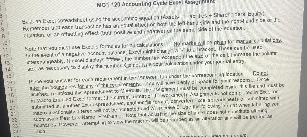
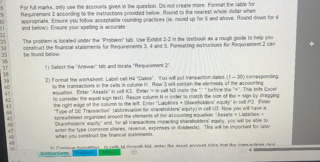
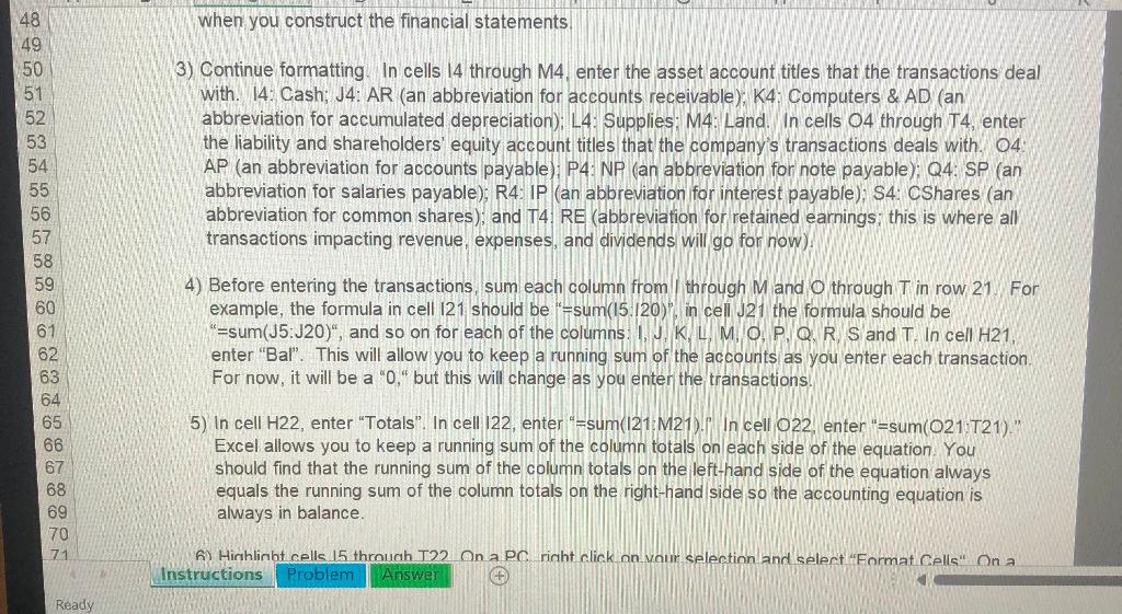
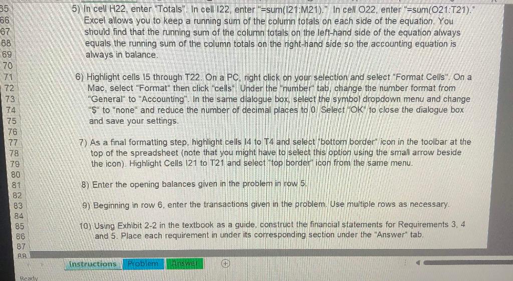
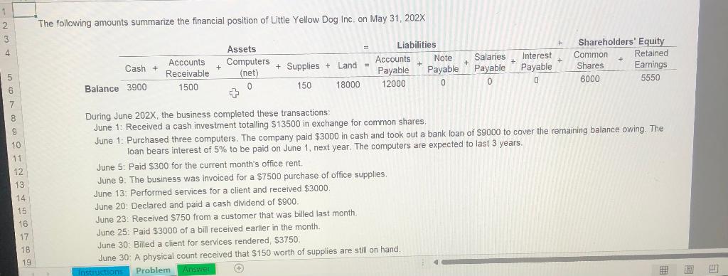
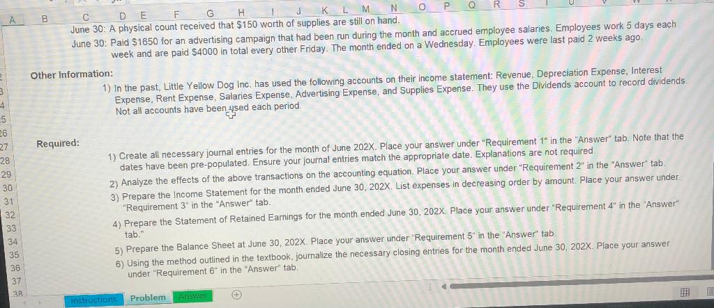
MGT 120 Accounting Cycle Excel Assignment Build an Excel spreadsheet using the accounting equation (Assets = Liabilities + Shareholders' Equity). Remember that each transaction has an equal effect on both the left-hand side and the right-hand side of the equation, or an offsetting effect (both positive and negative) on the same side of the equation. 5 3 7 8 9 10 11 12 13 14 15 16 17 18 19 20 21 22 23 24 Note that you must use Excel's formulas for all calculations. No marks will be given for manual calculations. In the event of a negative account balance, Excel might change a "-* to a bracket. These can be used interchangeably. If excel displays "****", the number has exceeded the size of the cell. Increase the column size as necessary to display the number. not type your calculation under your journal entry, Place your answer for each requirement in the "Answer" tab under the corresponding location. Do not alter the boundaries for any of the requirements. You will have plenty of space for your response. Once finished, re-upload this spreadsheet to Quercus. The assignment must be completed inside this file and must be in Macro Enabled Excel format (the current format of the worksheet). Assignments not completed in Excel or submitted in: another Excel spreadsheet, another file format, converted Excel spreadsheets or submitted with macro functionality altered will not be accepted and will receive 0. Use the following format when labelling your submission files: LastName, FirstName. Note that adjusting the size of a cell does not constitute altering boundries. However, attempting to view the macros will be recorded as an alteration and will be treated as such hleted as a group For full marks, only use the accounts given in the question. Do not create more. Format the table for Requirement 2 according to the instructions provided below. Round to the nearest whole dollar when appropriate. Ensure you follow acceptable rounding practices (ie. round up for 5 and above. Round down for 4 and below). Ensure your spelling is accurate, 8 -9 30 31 32 33 34 35 36 37 38 The problem is located under the "Problem" tab. Use Exhibit 2-2 in the textbook as a rough guide to help you construct the financial statements for Requirements 3, 4 and 5. Formatting instructions for Requirement 2 can be found below. 1) Select the "Answer" tab and locate "Requirement 2". 42 2) Format the worksheet. Label cell H4 "Dates". You will put transaction dates (1 - 30) corresponding to the transactions in the cells in column H. Row 3 will contain the elements of the accounting equation. Enter "Assets" in cell K3. Enter '= in cell N3 (note the "before the "="This tells Excel to consider the equal sign text). Resize column N in order to match the size of the = sign by dragging the right edge of the column to the left. Enter "Liabilities + Shareholders' equity" in cell P3. Enter "Type of SE Transaction" (abbreviation for shareholders' equity) in cell U3. Now you will have a spreadsheet organized around the elements of the accounting equation: "Assets = Liabilities + Shareholders' equity" and, for all transactions impacting shareholders' equity, you will be able to enter the type (common shares, revenue, expenses or dividends). This will be important for later when you construct the financial statements. 44 45 3) Continue formattina In cells. 14 through M4 enter the asset account titles that the transactions deal Instructions Problem Answer + when you construct the financial statements 50 3) Continue formatting. In cells 14 through M4, enter the asset account titles that the transactions deal with. 14. Cash; J4: AR (an abbreviation for accounts receivable), K4: Computers & AD (an abbreviation for accumulated depreciation); L4: Supplies: M4: Land. In cells 04 through T4, enter the liability and shareholders' equity account titles that the company's transactions deals with. 04 AP (an abbreviation for accounts payable): P4: NP (an abbreviation for note payable); Q4: SP (an abbreviation for salaries payable); R4: IP (an abbreviation for interest payable); S4: CShares (an abbreviation for common shares), and T4 RE (abbreviation for retained earnings: this is where all transactions impacting revenue, expenses, and dividends will go for now) NO:98% 2 3 397 98 good 4) Before entering the transactions, sum each column from through M and through T in row 21. For example, the formula in cell 121 should be "=sum(15.120), in cell J21 the formula should be "=sum(J5:J20)", and so on for each of the columns. I. K, L, M, O, P, Q, R S and T. In cell H21. enter "Bal". This will allow you to keep a running sum of the accounts as you enter each transaction, For now, it will be a "0." but this will change as you enter the transactions. 5) In cell H22, enter "Totals". In cell 122, enter"=sum(121 M21. In cell 022, enter "=sum(021 T21)." Excel allows you to keep a running sum of the column totals on each side of the equation. You should find that the running sum of the column totals on the left-hand side of the equation always equals the running sum of the column totals on the right-hand side so the accounting equation is always in balance. 6) Highlinbt cells 15 through T22 On a PC right click on your selection and select Format Cells". Ona Instructions Problem Answer Ready 5) In cell H22, enter "Totals". In cell 122, enter "=sum(121:M21). In cell 022, enter"=sum(021.T21)." Excel allows you to keep a running sum of the column totals on each side of the equation. You should find that the running sum of the column totals on the left-hand side of the equation always equals the running sum of the column totals on the right-hand side so the accounting equation is always in balance. 6) Highlight cells 15 through T22. On a PC, right click on your selection and select "Format Cells". On a Mac, select "Format" then click "cells". Under the "number tab, change the number format from "General to "Accounting". In the same dialogue box, select the symbol dropdown menu and change "S to none and reduce the number of decimal places to 0 Select "OK" to close the dialogue box and save your settings. 35 66 67 -68 69 70 71 72 73 74 75 76 77 78 79 80 81 82 83 84 85 86 87 88 7) As a final formatting step, highlight cells 14 to T4 and select "bottom border" icon in the toolbar at the top of the spreadsheet (note that you might have to select this option using the small arrow beside the icon). Highlight Cells 121 to T21 and select "top border" icon from the same menu. 8) Enter the opening balances given in the problem in row 5. 9) Beginning in row 6, enter the transactions given in the problem. Use multiple rows as necessary. 10) Using Exhibit 2-2 in the textbook as a guide, construct the financial statements for Requirements 3, 4 and 5. Place each requirement in under its corresponding section under the "Answer" tab. Instructions Problem Answer + Ready 1 2 3 The following amounts summarize the financial position of Little Yellow Dog Inc. on May 31, 202X 4 + + + + Cash + + Assets Computers (net) 0 + Supplies + Land = Liabilities + Accounts Note Salaries Interest + Payable Payable Payable Payable 12000 0 0 0 0 0 Shareholders' Equity Common Retained Shares Earnings 6000 5550 Accounts Receivable 1500 5 Balance 3900 150 18000 6 7 8 9 10 11 12 13 14 15 16 17 18 19 During June 202X, the business completed these transactions: June 1: Received a cash investment totalling $13500 in exchange for common shares June 1: Purchased three computers. The company paid $3000 in cash and took out a bank loan of S9000 to cover the remaining balance owing. The loan bears interest of 5% to be paid on June 1. next year. The computers are expected to last 3 years. June 5: Paid $300 for the current month's office rent. June 9: The business was invoiced for a $7500 purchase of office supplies. June 13: Performed services for a client and received $3000. June 20: Declared and paid a cash dividend of $900. June 23: Received $750 from a customer that was billed last month. June 25: Paid $3000 of a bill received earlier in the month June 30: Billed a client for services rendered, $3750. June 30: A physical count received that $150 worth of supplies are still on hand Instructions Problem Ansve! A B D E F G K L M N 0 Q R June 30: A physical count received that $150 worth of supplies are still on hand. June 30: Paid $1650 for an advertising campaign that had been run during the month and accrued employee salaries. Employees work 5 days each week and are paid $4000 in total every other Friday. The month ended on a Wednesday. Employees were last paid 2 weeks ago Other Information: 1) In the past, Little Yellow Dog Inc. has used the following accounts on their income statement: Revenue, Depreciation Expense, Interest Expense, Rent Expense, Salaries Expense, Advertising Expense, and Supplies Expense. They use the Dividends account to record dividends. Not all accounts have been used each period. Required: 4 -5 26 27 28 29 30 31 32 33 34 35 36 37 38 1) Create all necessary journal entries for the month of June 202X. Place your answer under "Requirement 1" in the "Answer tab. Note that the dates have been pre-populated. Ensure your journal entries match the appropriate date. Explanations are not required. 2) Analyze the effects of the above transactions on the accounting equation. Place your answer under "Requirement 2" in the "Answer" tab. 3) Prepare the Income Statement for the month ended June 30, 202X. List expenses in decreasing order by amount. Place your answer under "Requirement 3" in the "Answer" tab. 4) Prepare the Statement of Retained Earnings for the month ended June 30, 202X. Place your answer under "Requirement 4" in the "Answer tab. 5) Prepare the Balance Sheet at June 30, 202X. Place your answer under "Requirement 5" in the "Answer" tab. 6) Using the method outlined in the textbook, journalize the necessary closing entries for the month ended June 30, 202X. Place your answer under "Requirement 6" in the "Answer" tab. E instructions