Please solve with python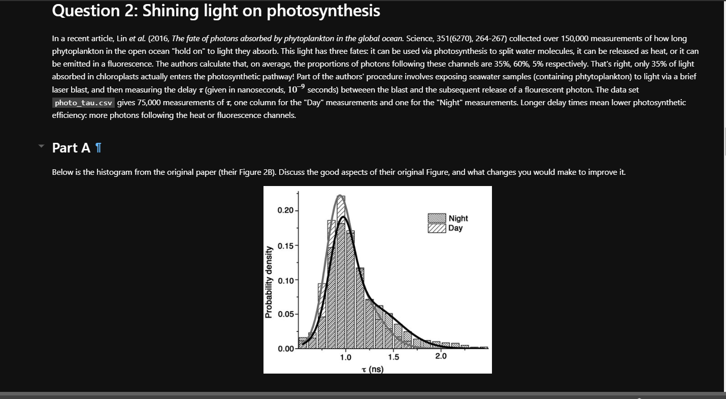

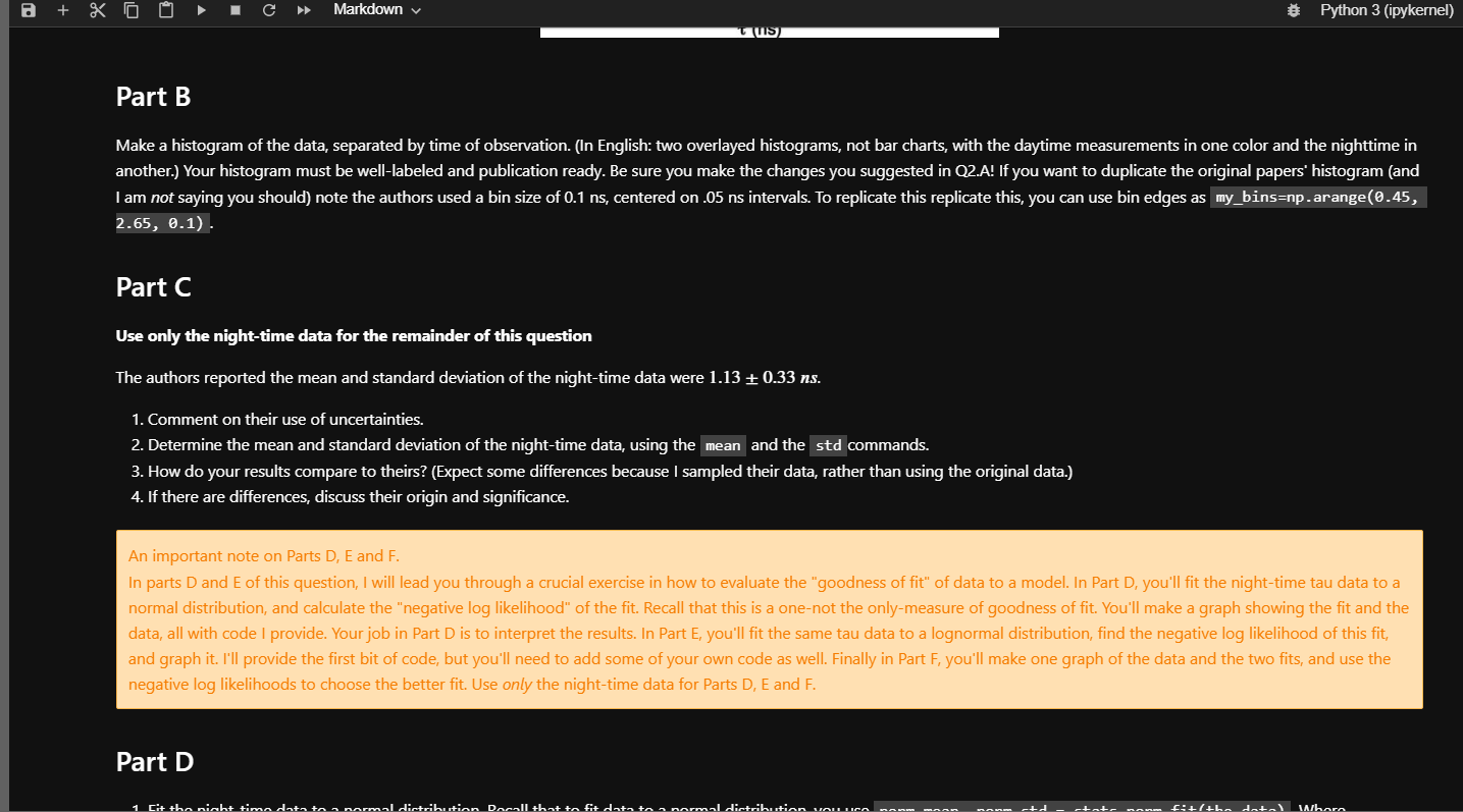
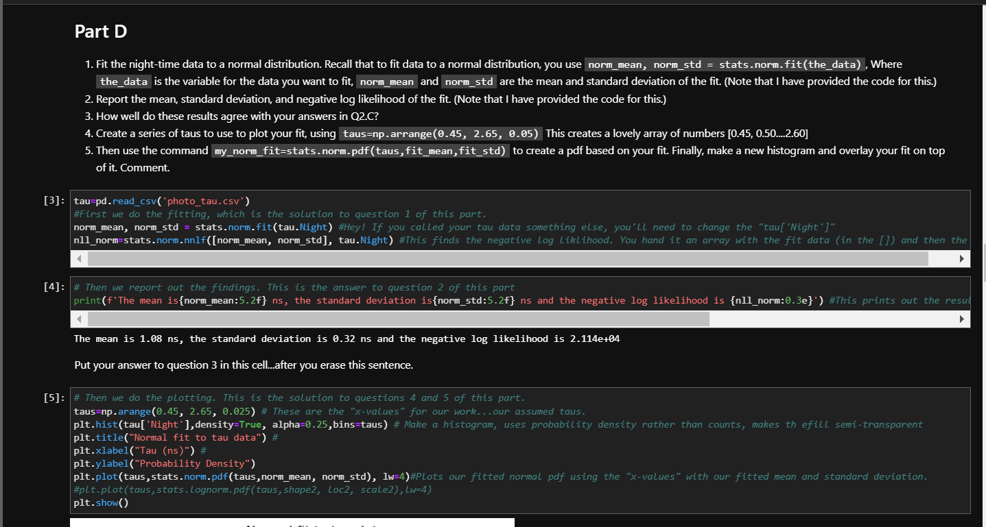
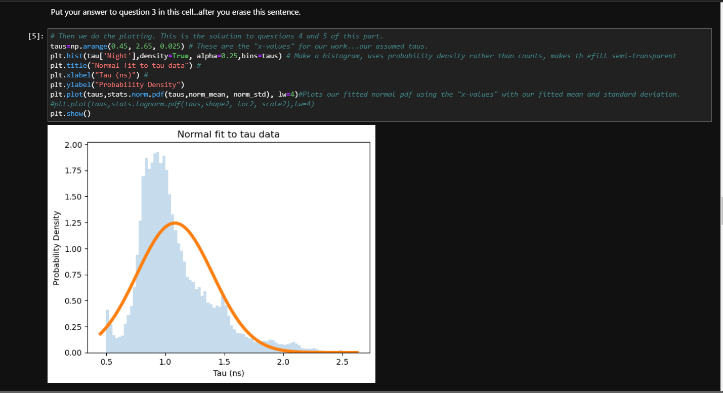
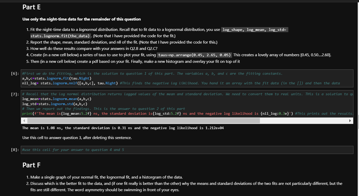
Question 2: Shining light on photosynthesis In a recent article, Lin et al. (2016, The fate of photons absorbed by phytoplankton in the global ocean. Science, 351(6270), 264-267) collected over 150,000 measurements of how long phytoplankton in the open ocean "hold on" to light they absorb. This light has three fates: it can be used via photosynthesis to split water molecules, it can be released as heat, or it can be emitted in a fluorescence. The authors calculate that, on average, the proportions of photons following these channels are 35%,60%,5% respectively. That's right, only 35% of light absorbed in chloroplasts actually enters the photosynthetic pathway! Part of the authors' procedure involves exposing seawater samples (containing phtytoplankton) to light via a brief laser blast, and then measuring the delay (given in nanoseconds, 109 seconds) betweeen the blast and the subsequent release of a flourescent photon. The data set photo_tau. csv gives 75,000 measurements of , one column for the "Day" measurements and one for the "Night" measurements. Longer delay times mean lower photosynthetic efficiency: more photons following the heat or fluorescence channels. Make a histogram of the data, separated by time of observation. (In English: two overlayed histograms, not bar charts, with the daytime measurements in one color and the nighttime in another.) Your histogram must be well-labeled and publication ready. Be sure you make the changes you suggested in Q2.A! If you want to duplicate the original papers' histogram (and I am not saying you should) note the authors used a bin size of 0.1ns, centered on .05ns intervals. To replicate this replicate this, you can use bin edges as my bins= 0.45 , 2.65,0.1) Part C Use only the night-time data for the remainder of this question The authors reported the mean and standard deviation of the night-time data were 1.130.33ns. 1. Comment on their use of uncertainties. 2. Determine the mean and standard deviation of the night-time data, using the mean and the std commands. 3. How do your results compare to theirs? (Expect some differences because I sampled their data, rather than using the original data.) 4. If there are differences, discuss their origin and significance. An important note on Parts D1,a and F. In parts D and E of this question, I will lead you through a crucial exercise in how to evaluate the "goodness of fit" of data to a model. In Part D, you'll fit the night-time tau data to a normal distribution, and calculate the "negative log likelihood" of the fit. Recall that this is a one-not the only-measure of goodness of fit. You'll make a graph showing the fit and the data, all with code I provide. Your job in Part D is to interpret the results. In Part E, you'll fit the same tau data to a lognormal distribution, find the negative log likelihood of this fit, and graph it. I'll provide the first bit of code, but you'll need to add some of your own code as well. Finally in Part F, you'll make one graph of the data and the two fits, and use the negative log likelihoods to choose the better fit. Use only the night-time data for Parts D,E and F. Part D 1. Fit the night-time data to a normal distribution. Recall that to fit data to a normal distribution, you use norm_mean, norm_std = stats.norm. fit (the_data) , Where 2. Report the mean, standard deviation, and negative log likelihood of the fit. (Note that I have provided the code for this.) 3. How well do these results agree with your answers in Q2.C? 4. Create a series of taus to use to plot your fit, using taus=np.arrange (0.45,2.65,0.05) This creates a lovely array of numbers [0.45,0.50...2.60] 5. Then use the command my_norm_fit=stats.norm.pdf(taus,_fit_mean,fit_std) to create a pdf based on your fit. Finally, make a new histogram and overlay your fit on top of it. Comment. tau = pd.read_csv( \#First we do the fitting, which is the solution to question 1 of this part. norm_mean, norm_std = stats.norm. fit(tau.Night) \#Hey! If you called your tau data something else, you'll need to change the "tau['Night']" \# Then we report out the findings. This is the answer to question 2 of this part The mean is 1.08ns, the standard deviation is 0.32 ns and the negative log likelihood is 2.114e+04 Put your answer to question 3 in this cell...after you erase this sentence. \# Then we do the plotting. This is the solution to questions 4 and 5 of this part. taus=np.arange (0.45,2.65,0.025) \# These are the "x-values" for our work...our assumed taus. plt.title("Normal fit to tau data") \# plt.xlabel("Tau (ns)") \# plt.ylabel("Probability Density") \#plt.plot(taus, stats. Lognorm.pdf(taus, shape2, loc2, scale2), (w=4) plt. show() Put your answer to question 3 in this cell...after you erase this sentence. Part E Use only the night-time data for the remainder of this question 1. Fit the night-time data to a lognormal distribution. Recall that to fit data to a lognormal distribution, you use log_shape, log_mean, log_std= stats. lognorm.fit(the_data). (Note that I have provided the code for the fit.) 2. Report the shape, mean, standard deviation, and nll of the fit. (Note that I have provided the code for this.) 3. How well do these results compare with your answers in Q2.B and Q2.C? 5. Then (in a new cell below) create a pdf based on your fit. Finally, make a new histogram and overlay your fit on top of it \#First we do the fitting, which is the solution to question 1 of this part. The variables a, b, and c are the fitting constants. a, b, c=stats. lognorm. fit(tau. Night) log_mean=stats. lognorm.mean(a,b,c) log_std=stats. lognorm.std (a,b,c) \# Then we report out the findings. This is the answer to question 2 of this part The mean is 1.08ns, the standard deviation is 0.31 ns and the negative loglikelihood is 1.212e+04 Use this cell to answer question 3 , after deleting this sentence. : \#use this cell for your answer to question 4 and 5 Part F 1. Make a single graph of your normal fit, the lognormal fit, and a historgram of the data. fits are still different. The word asymmetry should be swimming in front of your eyes