Please walk me through steps 8-13

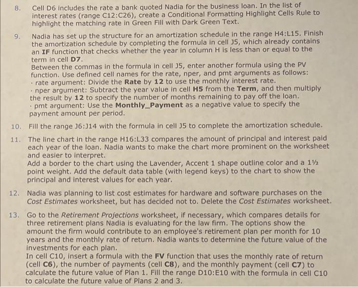
8. Cell D6 includes the rate a bank quoted Nadia for the business loan. In the list of interest rates (range C12:C26 ), create a Conditional Formatting Highlight Cells Rule to highlight the matching rate in Green Fill with Dark Green Text. 9. Nadia has set up the structure for an amortization schedule in the range H4:L15. Finish the amortization schedule by completing the formula in cell 35 , which already contains an IF function that checks whether the year in column H is less than or equal to the term in cell D7. Between the commas in the formula in cell 35 , enter another formula using the PV function. Use defined cell names for the rate, nper, and pmt arguments as follows: - rate argument: Divide the Rate by 12 to use the monthly interest rate. - nper argument: Subtract the year value in cell H5 from the Term, and then multiply the result by 12 to specify the number of months remaining to pay off the loan. - pmt argument: Use the Monthly_Payment as a negative value to specify the payment amount per period. 10. Fill the range 36:314 with the formula in cell J5 to complete the amortization schedule. 11. The line chart in the range H16:L33 compares the amount of principal and interest paid each year of the loan. Nadia wants to make the chart more prominent on the worksheet and easier to interpret. Add a border to the chart using the Lavender, Accent 1 shape outline color and a 11/2 point weight. Add the default data table (with legend keys) to the chart to show the principal and interest values for each year. 12. Nadia was planning to list cost estimates for hardware and software purchases on the Cost Estimates worksheet, but has decided not to. Delete the Cost Estimates worksheet. 13. Go to the Retirement Projections worksheet, if necessary, which compares details for three retirement plans Nadia is evaluating for the law firm. The options show the amount the firm would contribute to an employee's retirement plan per month for 10 years and the monthly rate of return. Nadia wants to determine the future value of the investments for each plan. In cell C10, insert a formula with the FV function that uses the monthly rate of return (cell C6), the number of payments (cell C8), and the monthly payment (cell C7) to calculate the future value of Plan 1. Fill the range D10:E10 with the formula in cell C10 to calculate the future value of Plans 2 and 3