plssss this one and explain all the steps please

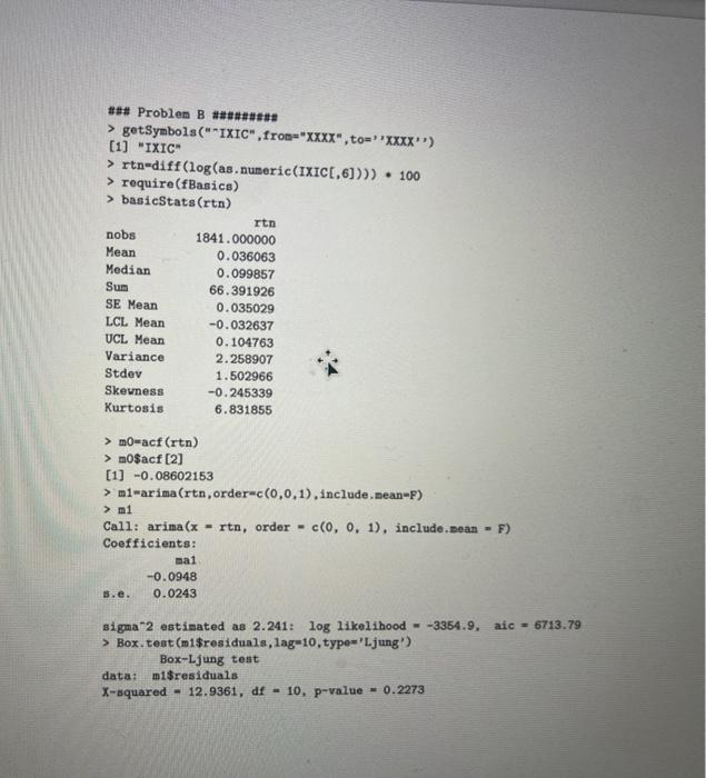
Question B (10 points) Consider the daily log returns n, in percentages, bf the NASDAQ index for a certain period of time with 1841 observations. Answer the following questions, using the attached R output. 1. Let u be the expected value of nt. Test Hoxu = 0 versus H: #0. Obtain the test statistic and draw your conclusion 2. Is the distribution of n skew? Why? 3. Does the distribution of n have heavy tails? Why? 4. Let pi be the lag-1 ACF of rt. Test Ho: p1 = 0 versus Hip#0. The sample lag-1 ACF is -0.086. Obtain the test statistic and draw your conclusion. 5. An MA(1) model is fitted. Write down the fitted model, including o2 of the residuals. ### Problem B ### > getSymbols("*IXIC" fron="XXXX", to="*XXXX) [1] "IXIC > rtn-diff(log(as. numeric(IXIC[,6]))) . 100 > require(fBasics) > basicStats (run) rtn nobs Mean Median Sum SE Mean LCL Mean UCL Mean Variance Stdev Skewness Kurtosis 1841.000000 0.036063 0.099857 66.391926 0.035029 -0.032637 0.104763 2.258907 1.502966 -0.245339 6.831855 > m-acf (rtn) > m0$acf [2] [1] -0.08602153 > mi-arima (rtn, order-c(0,0,1), include.mean-F) > m1 Call: arima (x - rtn, order- c(0, 0, 1), include.Dean - F) Coefficients: ma1 -0.0948 s.e. 0.0243 sigma2 estimated as 2.241: log likelihood --3354.9, aic - 6713.79 > Box.test(m1$residuals, lag=10, type='Ljung' Box-Ljung test data: m1$residuals X-squared - 12.9361, df - 10, p-value - 0.2273 Consider the daily log returns n, in percentages, of the NASDAQ index for a certain period of time with 1841 observations. Answer the following questions, using the attached R output. 1. Let u be the expected value of rt. Test Ho: u = 0 versus Ha : u 70. Obtain the test statistic and draw your conclusion. . 2. Is the distribution of n skew? Why? 3. Does the distribution of rt have heavy tails? Why? 4. Let pi be the lag-1 ACF of rt. Test Ho: p1 = 0 versus Ha: P80. The sample lag-1 ACF is -0.086. Obtain the test statistic and draw your conclusion. 5. An MA(1) model is fitted. Write down the fitted model, including 02 of the residuals. ### Problem B ######### > getSymbols("*IXIC", from="XXXX", to="XXXX'') [1] "IXIC" > rtn=diff(log(as. numeric(IXICC, 6]))) * 100 > require(fBasics) > basicStats (rtn) rtn nobs 1841.000000 Mean 0.036063 Median 0.099857 Sum 66.391926 SE Mean 0.035029 LCL Mean -0.032637 UCL Mean 0.104763 Variance 2.258907 Stdev 1.502966 Skewness -0.245339 Kurtosis 6.831855 > mo-acf (rtn) > mo$acf [2] [1] -0.08602153 > m1-arima (rtn,order=c(0,0,1), include.mean=F) > m1 Call: arima(x = rtn, order c(0, 0, 1), include.mean Coefficients: ma1 -0.0948 s.e. 0.0243 F) sigma 2 estimated as 2.241: log likelihood = -3354.9, aic - 6713.79 > Box.test(m1$residuals, lag=10, type='Ljung') Box-Ljung test data: m1$residuals X-squared = 12.9361, df = 10, p-value 0.2273 Question B (10 points) Consider the daily log returns n, in percentages, bf the NASDAQ index for a certain period of time with 1841 observations. Answer the following questions, using the attached R output. 1. Let u be the expected value of nt. Test Hoxu = 0 versus H: #0. Obtain the test statistic and draw your conclusion 2. Is the distribution of n skew? Why? 3. Does the distribution of n have heavy tails? Why? 4. Let pi be the lag-1 ACF of rt. Test Ho: p1 = 0 versus Hip#0. The sample lag-1 ACF is -0.086. Obtain the test statistic and draw your conclusion. 5. An MA(1) model is fitted. Write down the fitted model, including o2 of the residuals. ### Problem B ### > getSymbols("*IXIC" fron="XXXX", to="*XXXX) [1] "IXIC > rtn-diff(log(as. numeric(IXIC[,6]))) . 100 > require(fBasics) > basicStats (run) rtn nobs Mean Median Sum SE Mean LCL Mean UCL Mean Variance Stdev Skewness Kurtosis 1841.000000 0.036063 0.099857 66.391926 0.035029 -0.032637 0.104763 2.258907 1.502966 -0.245339 6.831855 > m-acf (rtn) > m0$acf [2] [1] -0.08602153 > mi-arima (rtn, order-c(0,0,1), include.mean-F) > m1 Call: arima (x - rtn, order- c(0, 0, 1), include.Dean - F) Coefficients: ma1 -0.0948 s.e. 0.0243 sigma2 estimated as 2.241: log likelihood --3354.9, aic - 6713.79 > Box.test(m1$residuals, lag=10, type='Ljung' Box-Ljung test data: m1$residuals X-squared - 12.9361, df - 10, p-value - 0.2273 Consider the daily log returns n, in percentages, of the NASDAQ index for a certain period of time with 1841 observations. Answer the following questions, using the attached R output. 1. Let u be the expected value of rt. Test Ho: u = 0 versus Ha : u 70. Obtain the test statistic and draw your conclusion. . 2. Is the distribution of n skew? Why? 3. Does the distribution of rt have heavy tails? Why? 4. Let pi be the lag-1 ACF of rt. Test Ho: p1 = 0 versus Ha: P80. The sample lag-1 ACF is -0.086. Obtain the test statistic and draw your conclusion. 5. An MA(1) model is fitted. Write down the fitted model, including 02 of the residuals. ### Problem B ######### > getSymbols("*IXIC", from="XXXX", to="XXXX'') [1] "IXIC" > rtn=diff(log(as. numeric(IXICC, 6]))) * 100 > require(fBasics) > basicStats (rtn) rtn nobs 1841.000000 Mean 0.036063 Median 0.099857 Sum 66.391926 SE Mean 0.035029 LCL Mean -0.032637 UCL Mean 0.104763 Variance 2.258907 Stdev 1.502966 Skewness -0.245339 Kurtosis 6.831855 > mo-acf (rtn) > mo$acf [2] [1] -0.08602153 > m1-arima (rtn,order=c(0,0,1), include.mean=F) > m1 Call: arima(x = rtn, order c(0, 0, 1), include.mean Coefficients: ma1 -0.0948 s.e. 0.0243 F) sigma 2 estimated as 2.241: log likelihood = -3354.9, aic - 6713.79 > Box.test(m1$residuals, lag=10, type='Ljung') Box-Ljung test data: m1$residuals X-squared = 12.9361, df = 10, p-value 0.2273