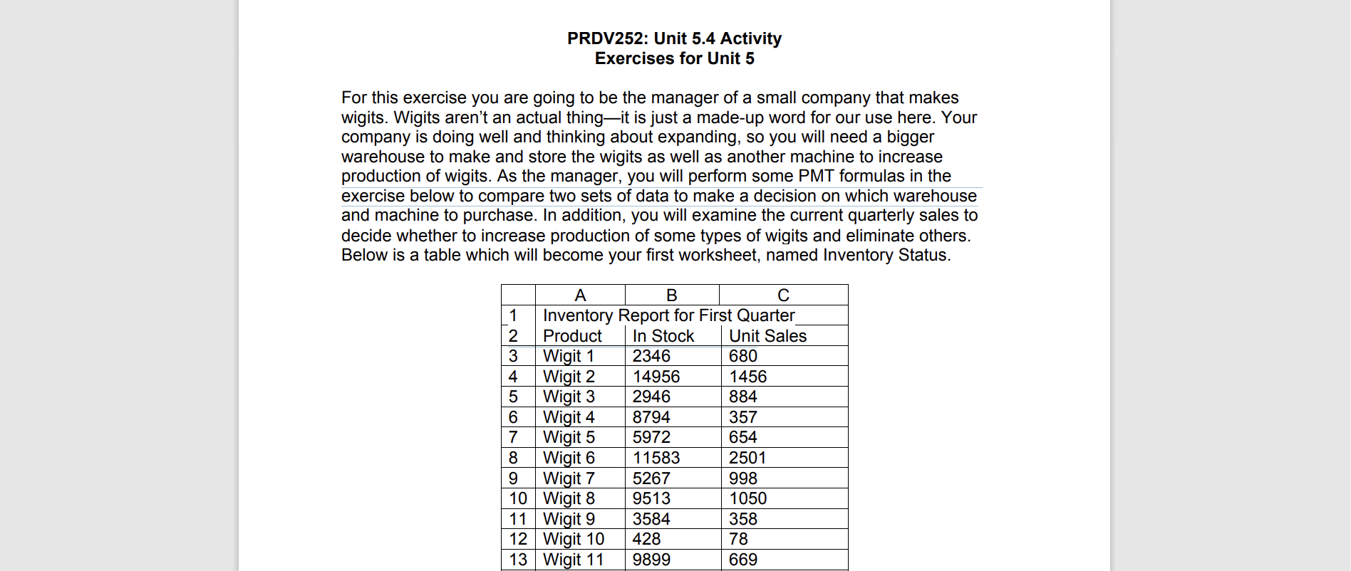
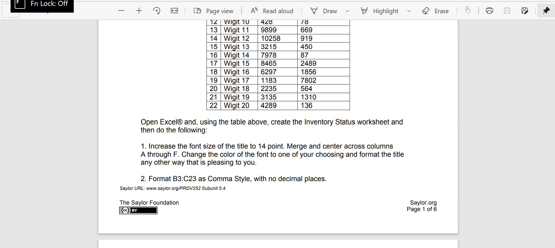
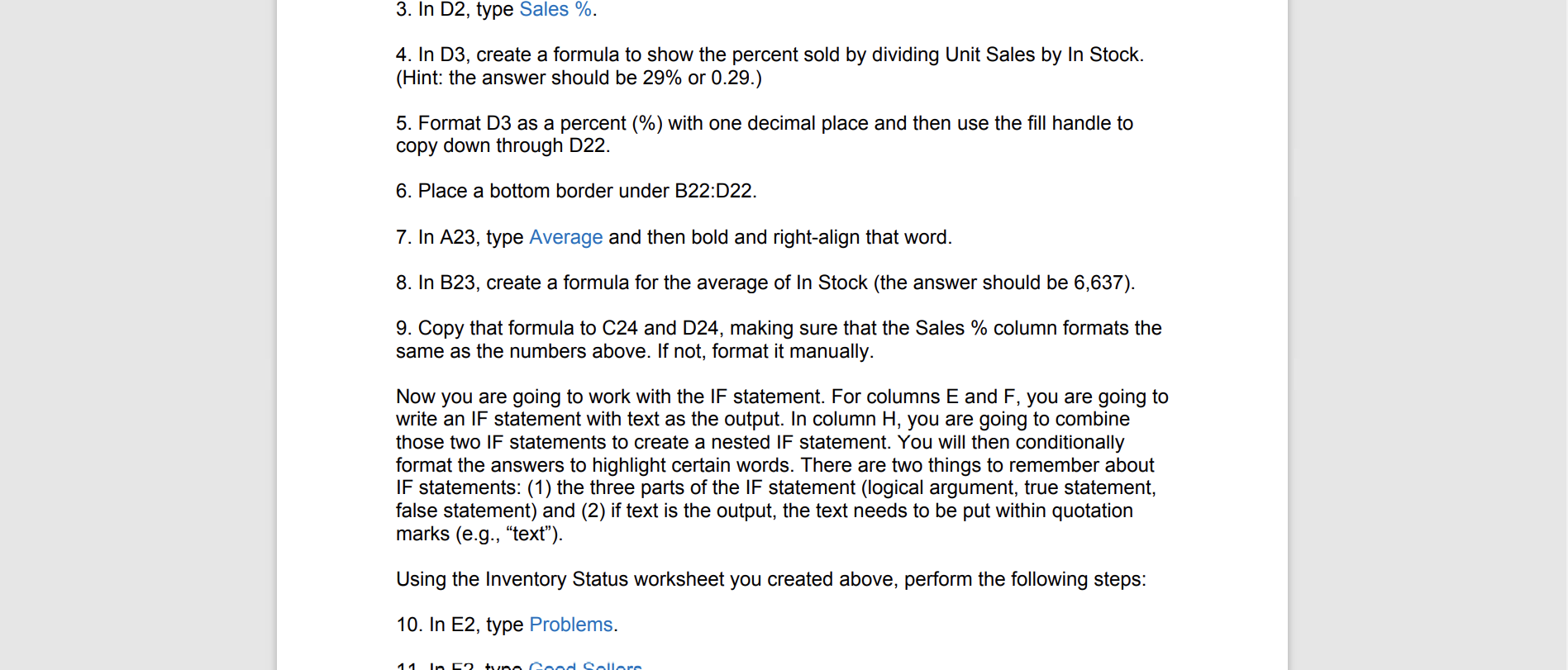
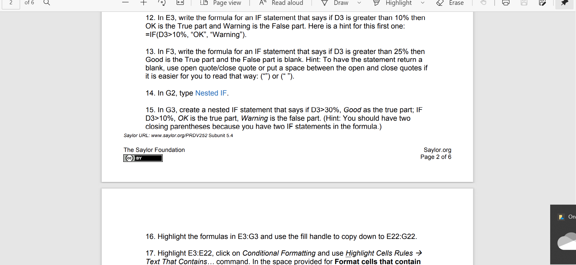
PRDV252: Unit 5.4 Activity Exercises for Unit 5 For this exercise you are going to be the manager of a small company that makes wigits. Wigits aren't an actual thingit is just a made-up word for our use here. Your company is doing well and thinking about expanding, so you will need a bigger warehouse to make and store the wigits as well as another machine to increase production of wigits. As the manager, you will perform some PMT formulas in the exercise below to compare two sets of data to make a decision on which warehouse and machine to purchase. In addition, you will examine the current quarterly sales to decide whether to increase production of some types of wigits and eliminate others. Below is a table which will become your first worksheet, named Inventory Status. A B 1 Inventory Report for First Quarter 2 Product In Stock Unit Sales 3 Wigit 1 2346 680 4 Wigit 2 14956 1456 5 Wigit 3 2946 884 6 Wigit 4 8794 357 7 Wigit 5 5972 654 8 Wigit 6 11583 2501 9 Wigit 7 5267 998 10 Wigit 8 9513 1050 11 Wigit 9 3584 358 12 Wigit 10 428 78 13 Wigit 11 9899 669 En Lock: Off Draw + Highlight Erase 19 78 669 919 450 {D Page view A Read aloud 12 Wigit 10 428 13 Wigit 11 9899 14 Wigit 12 10258 15 Wigit 13 3215 16 Wigit 14 7978 17 Wigit 15 8465 18 Wigit 16 6297 19 Wigit 17 1183 20 Wigit 18 2235 21 Wigit 19 3135 22 Wigit 20 4289 87 2489 1856 7802 564 1310 136 Open Excel and, using the table above, create the Inventory Status worksheet and then do the following: 1. Increase the font size of the title to 14 point. Merge and center across columns A through F. Change the color of the font to one of your choosing and format the title any other way that is pleasing to you. 2. Format B3:C23 as Comma Style, with no decimal places. Saylor URL: www.saylor.org/PRDV252 Subunit 5.4 The Saylor Foundation (CC BY Saylor.org Page 1 of 6 3. In D2, type Sales %. 4. In D3, create a formula to show the percent sold by dividing Unit Sales by In Stock. (Hint: the answer should be 29% or 0.29.) 5. Format D3 as a percent (%) with one decimal place and then use the fill handle to copy down through D22. 6. Place a bottom border under B22:D22. 7. In A23, type Average and then bold and right-align that word. 8. In B23, create a formula for the average of In Stock (the answer should be 6,637). 9. Copy that formula to C24 and D24, making sure that the Sales % column formats the same as the numbers above. If not, format it manually. Now you are going to work with the IF statement. For columns E and F, you are going to write an IF statement with text as the output. In column H, you are going to combine those two IF statements to create a nested IF statement. You will then conditionally format the answers to highlight certain words. There are two things to remember about IF statements: (1) the three parts of the IF statement (logical argument, true statement, false statement) and (2) if text is the output, the text needs to be put within quotation marks (e.g., "text"). Using the Inventory Status worksheet you created above, perform the following steps: 10. In E2, type Problems. 14 Csaed Collare 2 of 6 Q - + 1.D Page view A Read aloud Draw Highlight Erase o 12. In E3, write the formula for an IF statement that says if D3 is greater than 10% then OK is the True part and Warning is the False part. Here is a hint for this first one: =IF(D3>10%, OK, Warning). 13. In F3, write the formula for an IF statement that says if D3 is greater than 25% then Good is the True part and the False part is blank. Hint: To have the statement return a blank, use open quote/close quote or put a space between the open and close quotes if it is easier for you to read that way: () or ( ). 14. In G2, type Nested IF. 15. In G3, create a nested IF statement that says if D3>30%, Good as the true part; IF D3>10%, OK is the true part, Warning is the false part. (Hint: You should have two closing parentheses because you have two IF statements in the formula.) Saylor URL: www.saylor.org/PRDV252 Subunit 5.4 The Saylor Foundation CC BY Saylor.org Page 2 of 6 | On 16. Highlight the formulas in E3:G3 and use the fill handle to copy down to E22:G22. 17. Highlight E3:E22, click on Conditional Formatting and use Highlight Cells Rules Text That Contains... command. In the space provided for Format cells that contain 18. For Column G, conditionally format the columns using the Highlight Cells Rules Text That Contains... command. In the space provided for Format cells that contain the text:, type Warning, and in the space provided for with, select Red Text. 19. Again for Column G, repeat step 18 but use the word Good. Select Custom Format... and choose Bold as the Font style and dark blue as the Color. 20. In cell F24, type Number of products to reevaluate. You are going to create a COUNTIF formula to see how many of your wigits products need to be reevaluated so they can be either discontinued or given more effort with regard to sales. 21. In cell E24, create the COUNTIF statement using cells E3:E22 as the range and the word Warning as the criteria. Remember, because you are using text in this formula, the text must be within quotation marks. 22. Bold all of the column headings and center the headings in columns B through G. 23. Your finished worksheet will look similar to the image below