Question: Prepare the workbook as follows Create a new work book and save it as [ Your Name ] Boutique du Chic Year 1 Operating Budget
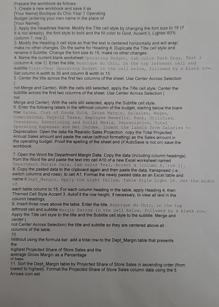
Prepare the workbook as follows
Create a new work book and save it as
Your Name Boutique du Chic Year Operating
Budget entering your cwn name in the place of Yout Name
Apply the Headlines theme. Modify the Title cell style by changing the font size to if it is not already? the font style to bold and the fill color to Gold, Accent Lighter oolumn row
Modify the Heading cell style so that the text is centered horizontally and will wrap; make no other changes. Do the samo for Heading Duplicate the Title cell style and rename it Subtitle Change the font size to ; make no other changes.
Name the current blank worksheet Operating Budges, tab color Dark Gray, Text column row Enter the title, Boutique du chic, in the top leftmost cell and subtile fitstYear Operating Budget in the cell below, followed by a blank zow. Set column A width to and column B width to
Center the title across the first two columns of the sheet Use Center Across Selection
not Merge and Center With the cells stil selected, apply the Title cell style. Center the subtitie across the first two columns of the sheet. Use Center Across Selection not
Merge and Center Whth the cells still selected, apply the Subelle cell style.
Enter the following labels in the leftmost column of the budget, starting below the blank
row, Sales, Cost of Goods Sold, Gross Marqin, Salaries, Wages,
Comiseions, Payroll axes, Employee Benefits, Rent, Veilities,
Insurance, Advertising and Soclal Medla, Depreciation, Total
Operating Expenses and Net Income, Indent the labels from Salaries to
Depreciation. Open the data file Realistic Sales Projection, copy the Total Projected
Annual Sales amount and paste the value without formatting as the Sales amount in the operating budget. Proof the spelling of the sheet and if AutoSave is not on save the workbook.
Open the Word file Department Margin Data. Copy the data including column headings from the Word file and paste the text into cell A of a new Excel worksheet named
Departhent Margin Data, tab color Teal, Accent & colunn row
Copy the pasted data to the clipboard again and then paste the data, transposed ie
switch columns and rows to cell A Format the newly pasted data as an Excel table and
name it DeptMargin. Apply the Light Yellow, Table Style Light Set the width of
each table column to For each column heading in the table, apply Heading then
Therned Cell Style Accent Autofit the row height, if necessary, to view all text in the column headings.
Insert three rows above the table. Enter the title, Boutique du chic, in the top
leftmost cell and subtitle Margin Ratios in the cell below, followed by a blank row.
Apply the Title cell style to the titie and the Subtesle cell style to the subtite. Merge and center
not Center Across Selection the title and subtille so they are centered above all columns of the table.
Without using the formula bar, add a total row to the DeptMargin table that presents the
highest Projected Share of Store Sales and the
average Gross Margin as a Percentage
of Siles.
Sort the DeptMargin table by Projected Share of Store Sales in ascending order from
lowest to highest Format the Projected Share of Store Sales column data using the
Arrows icon set.

Step by Step Solution
There are 3 Steps involved in it
1 Expert Approved Answer
Step: 1 Unlock


Question Has Been Solved by an Expert!
Get step-by-step solutions from verified subject matter experts
Step: 2 Unlock
Step: 3 Unlock


