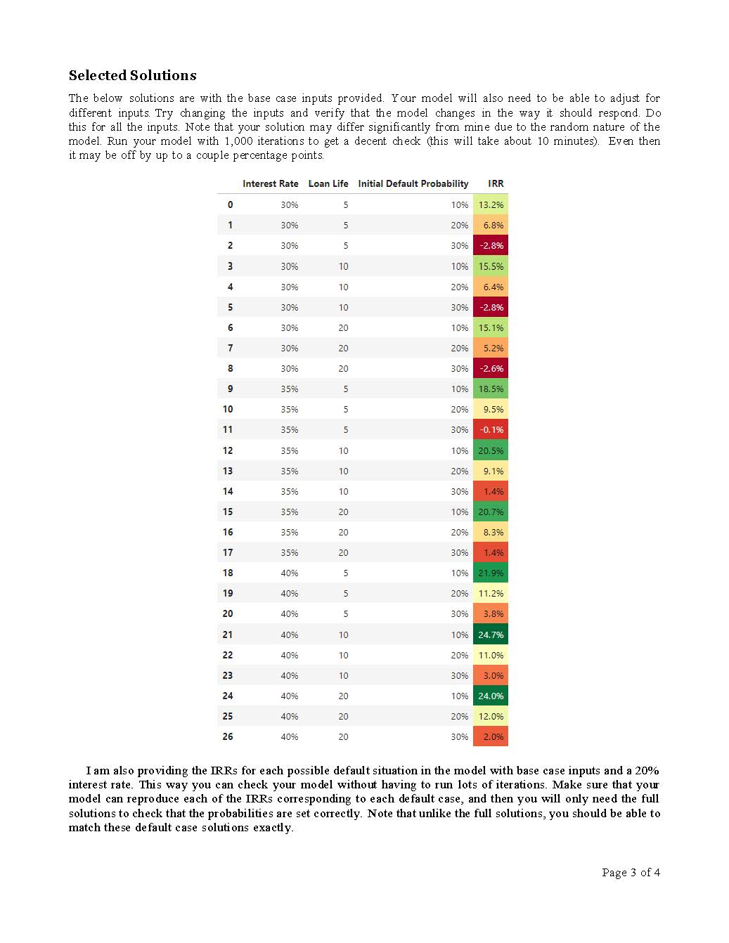
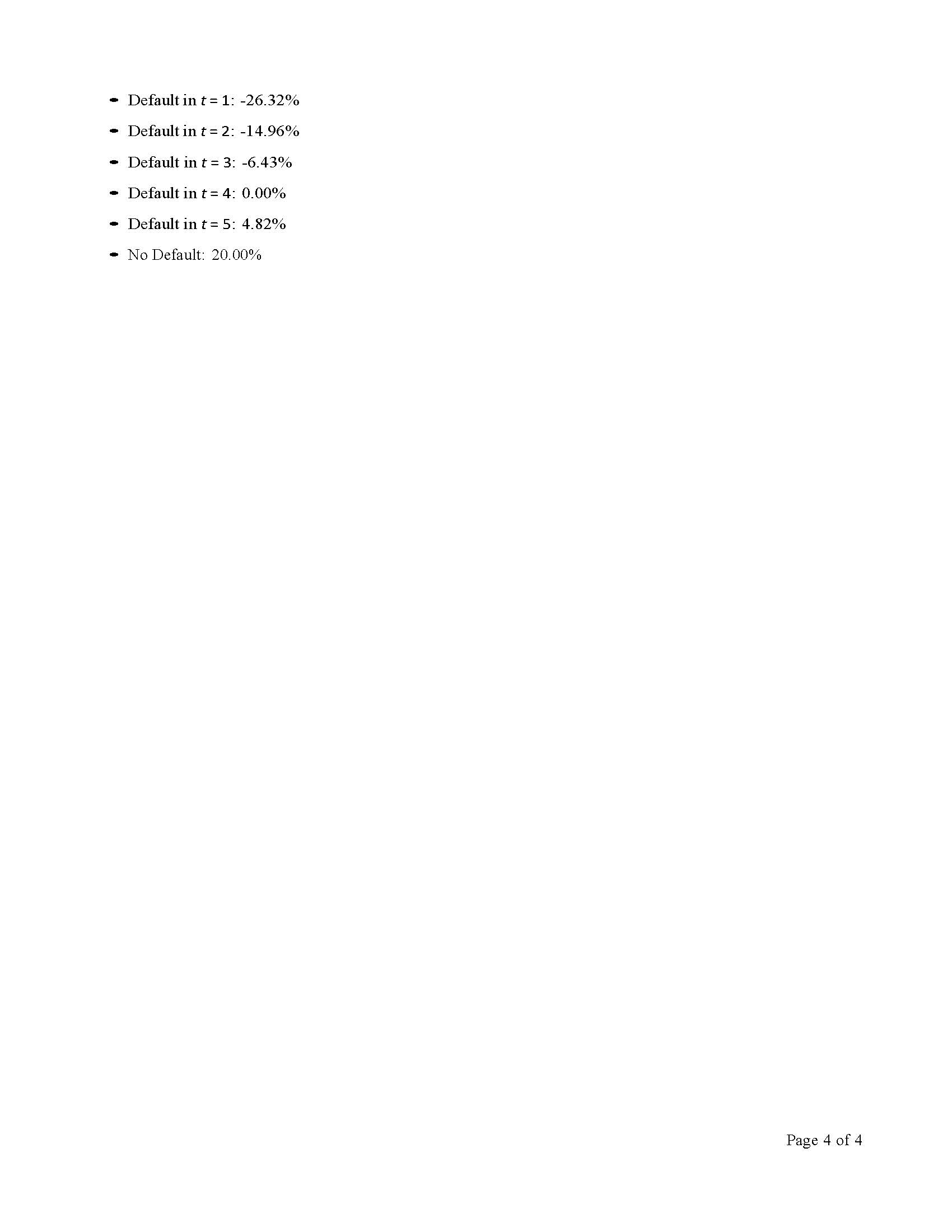
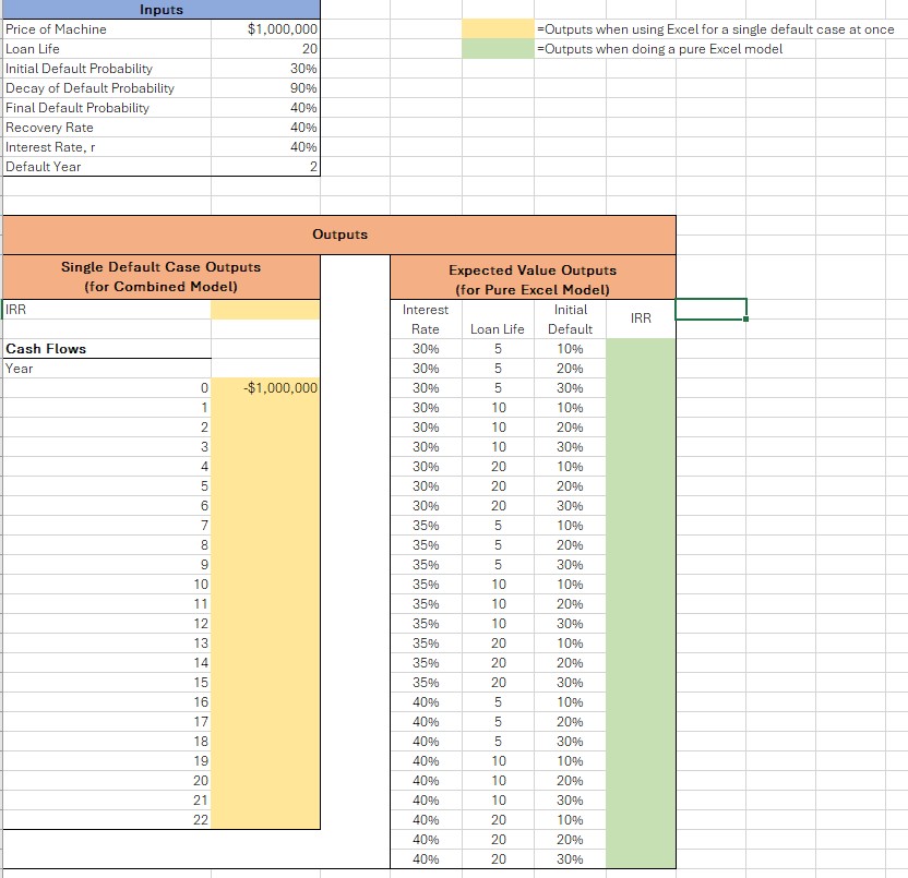
Probabilistic Loan Pricing Overview Problem Definition You work for a bank who is considering loaning funds to a small manufacturing business. The business needs pricemactine to buy machinery. The business would like to borrow the funds for nsr, and at that time it will Tepay Pricemacnine in full. Interest is paid annually at a rate of riareres: {(in the final period, both pricemachine and interest at the rate of riveress Will be paid). As this is a small business, there is significant default risk, but that default risk decreases over time as the business matures. The probability of default in the first year is p**, and then each year thereafter it is: prdefault o pff{au{tDecaydefau!t (1) Finally, the default probability is different in the final year, as it is the repayment year. The business has to pay a lot more in this period so there is a greater likelihood it can't come up with the funds. In the final year, (at year niire), the default probability is p?e@, When the business defaults, then the default covenants of the loan trigger bankruptcy for the borrower, and the borrower must pay as much as it can on the loan in the bankruptcy process. The bankruptcy process takes two years, and then once it 1s resolved, the lender will collect rrecovery% of pricemachine. For the year of default and the year after, the lender will not collect any cash flows, and then two years after default, the lender will collect FrecoveryPtiCemachine. INote that this means the number of vears of cash flows may be up to two years greater than the life of the loan. Main Question You are the commercial loan analyst trying to decide if this loan makes sense for the bank. You want to give the lending officer all the information she would need to negotiate a rate for this loan. Given the inputs, what is the expected IRR of the loan for a variety of interest rates on the loan? The lending officer would like you to evaluate rates in 5% increments from 30% to 40%. The lending officer is also worried that she may have estimated p* incorrectly. She is hoping for the answers to the above questions considering that p*\"* may vary. Evaluate the above questions for p?/**" = 0.1, 0.3 in addition to the base case of 0.2. Finally, the lending officer is unsure for how long she should extend the loan. So she would like to see all of the previously mentioned results with loan lifes of 5, 10, and 20 years. You should visualize the results of your model through graphs, conditional formatting, etc. Notes = You may assume a maximum loan life of 20 years in your model, which would make up to 22 years of cash flows. = Probably the easiest approach to building this model will use internal randomness. Though it certainly is possible to build this model using only expected values, T think that is generally more difficult. With the internal randomness approach, make sure you set the number of iterations to 1,000 per set of inputs to get a good estimate. While you are testing things out, set it lower, such as 10 or 100, to have it run quicker, but beware that the lower your number of iterations, the less consistent the results will be. Also beware that with 1,000 iterations as required for the final submission, it may take over an hour to run the model, so plan for that time. You may choose to either submit a pure Python model, pure Excel model, or a combination of the two. If you use both, then the Python model should be what I ultimately run and extract results from. The Python model would be running the Excel model many times and extracting the results. Upon reading the prior note, you may think to implement in pure Excel because of greater familiarity, but I think you will find meeting the objective of running the model repeatedly with three changing inputs quite difficult. You need to run your model 27,000 times in total with three inputs changing together. Your answers may differ slightly from those in the Selected Solutions section. This is the nature of a random model. They should be very close with 1,000 iterations, though. Do not move any of the input or output cells. Inputs 1. 2 3 Price machine: 1000000 el S ppefautt. 02 Decaydefaur: 0.9 pRefoult: 0.4 rrecovery i 0'4 Submission & Grading Submission Work off of the "Project 2 Template xlsx" and "Project 2 Template.ipynb\" files to my email. It is up to you whether you submit a pure Python, pure Excel, or combination model. For whichever tools you use, you should use the templates, so those submitting a combination model will submit both a Jupyter notebook and an Excel workbook, both based off the templates. With the combination model, your ultimate answer should be in the Jupyter notebook. Page 2 0f 4 Selected Solutions The below solutions are with the base case inputs provided. Your medel will also need to be able to adjust for different inputs Try changing the inputs and verify that the maodel changes in the way it should respond Do this for all the inputs. MNote that your solution may differ significantly from mine due to the random nature of the model. Run your model with 1,000 iterations to get a decent check (this will take about 10 minutes). ] it may be off by up to a couple percentage points Interest Rate Loan Life Initial Default Probability IRR 0 30% 5 10% 13.2% 1 30% 5 20% 6.8% 2 30% 5 305 R 3 309 10 109 | 15.5% 4 30% 10 20% | 6.4% 5 30% 10 205 R 6 20% 20 10% | 15.1% 7 30% 20 20% 526, 8 30% 20 aaea 9 35% 5 10% | 18.5% 10 35% 5 11 35% 5 12 35% 10 13 35% 10 14 35% 10 30% 15 35% 20 10% 16 35% 20 20% 8.3% 17 253 20 20% 18 40% 5 10% 19 40% 5 20 40% 5 21 40% 10 22 40% 10 23 40% 10 24 40% 20 25 40% 20 26 40% 20 Everl then Iam also providing the TRRs for each possible default situation in the model with base case inputs and a 20% interest rate. This way you can check your model without having to run lots of iterations. Make sure model can reproduce each of the IRRs corresponding to each default case, and then you will only nee that your d the full solutions to check that the probabilities are set correctly. Note that unlike the full solutions, you should be able to match these default case solutions exactly. Page 3 of 4 - Default in t = 1: -26.32% - Default in t = 2: -14.96% - Default in t = 3: -6.43% - Default in t = 4: 0.00% - Default in t = 5: 4.82% - No Default: 20.00% Page 4 of 4Inputs =Outputs when using Excel for a single default case at once Price of Machine $1,000,000 Loan Life 20 =Outputs when doing a pure Excel model Initial Default Probability 30% Decay of Default Probability 90% Final Default Probability 40% Recovery Rate 40% Interest Rate, 40% Default Year 2 Outputs Single Default Case Outputs Expected Value Outputs (for Combined Model) (for Pure Excel Model) Interest nitial IRR IBR Rate Loan Life Default Cash Flows 30% 5 10% 30% 20% Year $1,000,000 30% 30% 30% 10 10% 30% 10 20% 30% 10 30% 30% 20 10% 30% 20 20% 30% 20 30% 35% 10% 356 20% 35% 30% 3546 10 10% 11 356 10 20% 12 35% 10 30% 13 35% 20 10% 14 3546 20 20% 15 35% 20 30% 16 40% 5 10% 17 40% 20% 18 30% 19 40% 10 10% 20 40% 10 20% 21 40% 10 30% 22 4046 20 10% 40% 20 20% 40% 20 30%