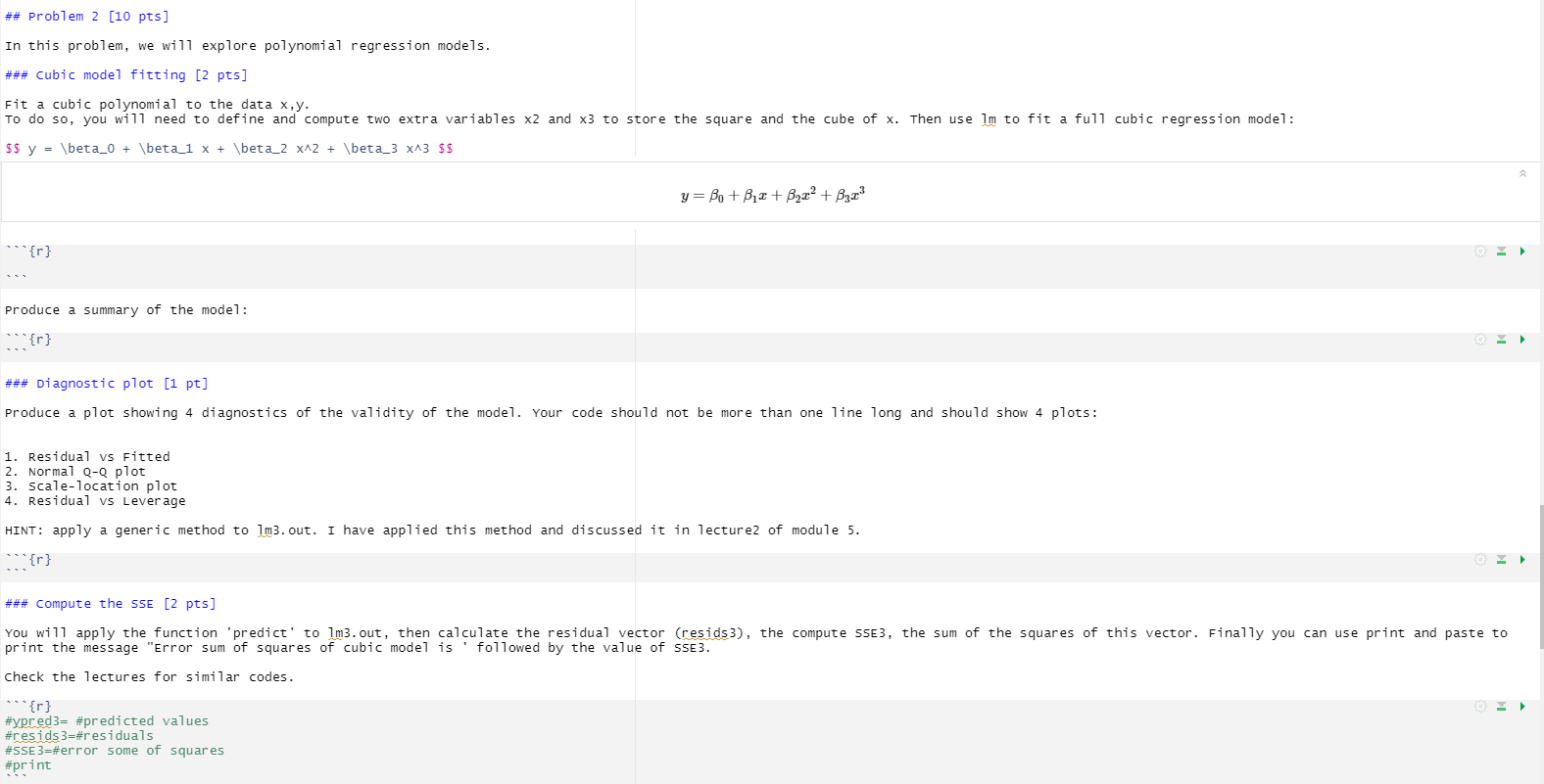
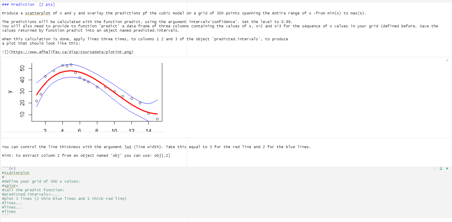
## Problem 2 [10 pts] In this problem, we will explore polynomial regression models. ### cubic model fitting [2 pts] Fit a cubic polynomial to the data x, y. To do so, you will need to define and compute two extra variables x2 and x3 to store the square and the cube of x. Then use Im to fit a full cubic regression model: $5 y = \\beta_0 + \\beta_1 x + \\beta_2 x42 + \\beta_3 x43 $$ y = Bo+ BI + B2x2 + B3x3 "{r} Produce a summary of the model: ### Diagnostic plot [1 pt] Produce a plot showing 4 diagnostics of the validity of the model. Your code should not be more than one line long and should show 4 plots: 1. Residual vs Fitted 2. Normal Q-Q plot 3. scale-location plot 4. Residual vs Leverage HINT: apply a generic method to 1m3. out. I have applied this method and discussed it in lecture2 of module 5. "{r} ### Compute the SSE [2 pts] You will apply the function 'predict' to 1m3. out, then calculate the residual vector (resids3), the compute SSE3, the sum of the squares of this vector. Finally you can use print and paste to print the message "Error sum of squares of cubic model is ' followed by the value of SSE3. check the lectures for similar codes. "{r} #ypred3= #predicted values #resids3=#residuals #SSE3=#error some of squares #print### Prediction [2 pts] Produce a scatterplot of x and y and overlay the predictions of the cubic model on a grid of 300 points spanning the entire range of x -from min(x) to max(x). The predictions will be calculated with the function predict, using the argument interval='confidence'. Set the level to 0. 99. You will also need to provide to function 'predict' a data frame of three columns containing the values of x, x42 and x43 for the sequence of x values in your grid (defined before. Save the values returned by function predict into an object named predicted. intervals. when this calculation is done, apply lines three times, to columns 1 2 and 3 of the object 'predicted. intervals', to produce a plot that should look like this: ! (https://www. afhalifax. ca/disp/coursedata/plotint. png) 10 20 30 40 50 6 10 14 You can control the line thickness with the argument 1wd (line width). Take this equal to 3 for the red line and 2 for the blue lines. Hint: to extract column 2 from an object named 'obj' you can use: obj [, 2] "{r} #scatterplot # #define your grid of 300 x values: #xplot= #call the predict function: #predicted. intervals