Problem #4 please

example 3.3.4

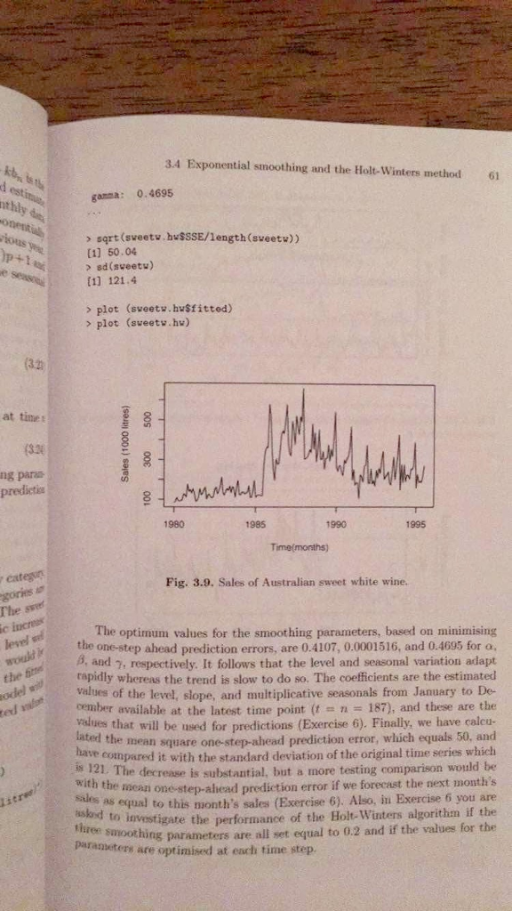
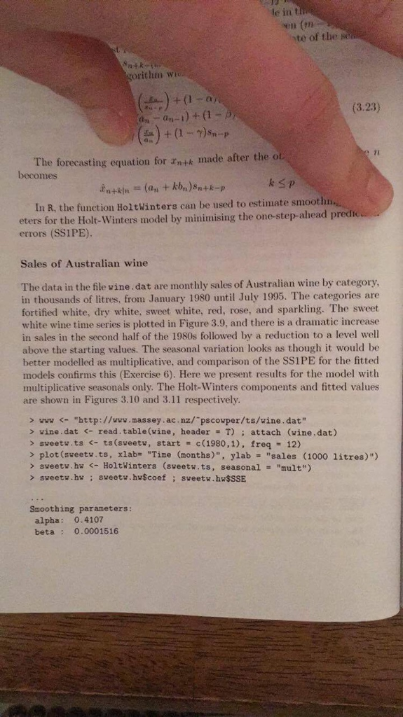
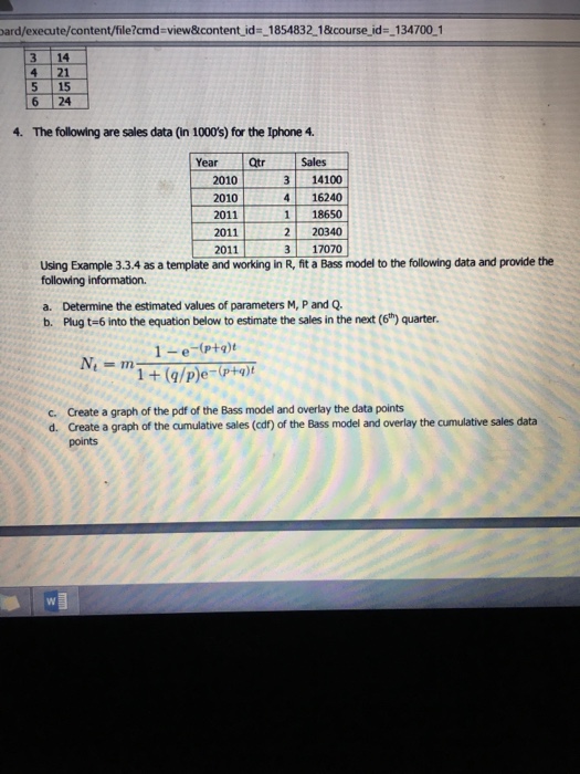
The following are sates data (In 1000's) for the I phone 4. Using Example 3.3.4 as a template and working in R, fit a Bass model to the following data and provide the following information. Determine the estimated values of parameters M, P and Q. Plug t=6 into the equation below to estimate the sales in the next (6^th) quarter. N_t = m 1 - e^-(p + q)^t/1 + (q/p)e^-(p + q)^t Create a graph of the pdf of the Bass model and overlay the data points Create a graph of the cumulative sales (cdf) of the Bass model and overlay the cumulative sales data points > sqrt(sweetw. hwSSSE/length(sweetw)) [1] 50 .04 > sd(sweetw) [1] 121.4 > plot (sweetw.) > plot (sweetw.hw) The optimum values for the smoothing parameters, based on minimizing the one-step ahead prediction errors, are 0.4107, 0.0001516, and 0.4095 for alpha, beta and respectively. It follows that the level and seasonal variation adapt rapidly whereas the trend is slow to do so. The coefficients are the estimated values of the level, slope, and multiplicative seasonal from January to December available at the latest time point (t = n = 187), and these are the values that will be used for predictions (Exercise 6). Finally, we have calculated the mean square one-step-ahead prediction error, which equals 50, and have compared it with the standard deviation of the original time series which is 121 The decrease is substantial, but a more testing comparison would be with the mean one-step-ahead prediction error if we forecast the next month's sales as equal to this month's sales (Exercise 6). Also, in Exercise 6 you are asked to investigate the performance of the Holt-Winters algorithm if the three smoothing parameters are all set equal to 0.2 and if the values for the parameters are optimized at each time step. The forecasting equation for x_n + k made after the becomes r_n + k|n = (a_n + kb_n)8_n + k - p k lessthanorequalto p In R, the function Holt Winters can be used to estimate smooth enters for the Holt-Winters model by minimising the one-step-ahead perch errors (SSIPE). Sales of Australian wine the data in the file wine.dat are monthly sales of Australian wine by category, in thousands of liters, from January 1980 until July 1995. The categories are fortified white, dry white, sweet white, red, rose, and sparkling. The sweet white wine time series is plotted in Figure 3.9. and there is a dramatic increase in sales in the second half of the 1980s followed by a reduction to a level well above the starting values. The seasonal variation looks as though it would be better modelled as multiplicative, and comparison of the SS1PE for the fitted models confirms this (Exercise 6). Here we present results for the model with multiplicative seasonal only. The Holt-Winters components and fitted values are shown in Figures 3.10 and 3.11 respectively. > www wine.dat sweetw.ts plot(sweetw.ts, xlab= "Time (months)", ylab - "sales (1000 litres)") > sweetw.hw sweetw.hw; sweetw.hw$coef; sweetw.hw$SSE Smoothing parameters: alpha: 0.4107 beta: 0.0001516 The following are sates data (In 1000's) for the I phone 4. Using Example 3.3.4 as a template and working in R, fit a Bass model to the following data and provide the following information. Determine the estimated values of parameters M, P and Q. Plug t=6 into the equation below to estimate the sales in the next (6^th) quarter. N_t = m 1 - e^-(p + q)^t/1 + (q/p)e^-(p + q)^t Create a graph of the pdf of the Bass model and overlay the data points Create a graph of the cumulative sales (cdf) of the Bass model and overlay the cumulative sales data points > sqrt(sweetw. hwSSSE/length(sweetw)) [1] 50 .04 > sd(sweetw) [1] 121.4 > plot (sweetw.) > plot (sweetw.hw) The optimum values for the smoothing parameters, based on minimizing the one-step ahead prediction errors, are 0.4107, 0.0001516, and 0.4095 for alpha, beta and respectively. It follows that the level and seasonal variation adapt rapidly whereas the trend is slow to do so. The coefficients are the estimated values of the level, slope, and multiplicative seasonal from January to December available at the latest time point (t = n = 187), and these are the values that will be used for predictions (Exercise 6). Finally, we have calculated the mean square one-step-ahead prediction error, which equals 50, and have compared it with the standard deviation of the original time series which is 121 The decrease is substantial, but a more testing comparison would be with the mean one-step-ahead prediction error if we forecast the next month's sales as equal to this month's sales (Exercise 6). Also, in Exercise 6 you are asked to investigate the performance of the Holt-Winters algorithm if the three smoothing parameters are all set equal to 0.2 and if the values for the parameters are optimized at each time step. The forecasting equation for x_n + k made after the becomes r_n + k|n = (a_n + kb_n)8_n + k - p k lessthanorequalto p In R, the function Holt Winters can be used to estimate smooth enters for the Holt-Winters model by minimising the one-step-ahead perch errors (SSIPE). Sales of Australian wine the data in the file wine.dat are monthly sales of Australian wine by category, in thousands of liters, from January 1980 until July 1995. The categories are fortified white, dry white, sweet white, red, rose, and sparkling. The sweet white wine time series is plotted in Figure 3.9. and there is a dramatic increase in sales in the second half of the 1980s followed by a reduction to a level well above the starting values. The seasonal variation looks as though it would be better modelled as multiplicative, and comparison of the SS1PE for the fitted models confirms this (Exercise 6). Here we present results for the model with multiplicative seasonal only. The Holt-Winters components and fitted values are shown in Figures 3.10 and 3.11 respectively. > www wine.dat sweetw.ts plot(sweetw.ts, xlab= "Time (months)", ylab - "sales (1000 litres)") > sweetw.hw sweetw.hw; sweetw.hw$coef; sweetw.hw$SSE Smoothing parameters: alpha: 0.4107 beta: 0.0001516