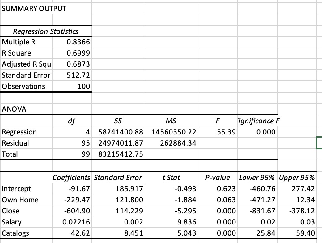
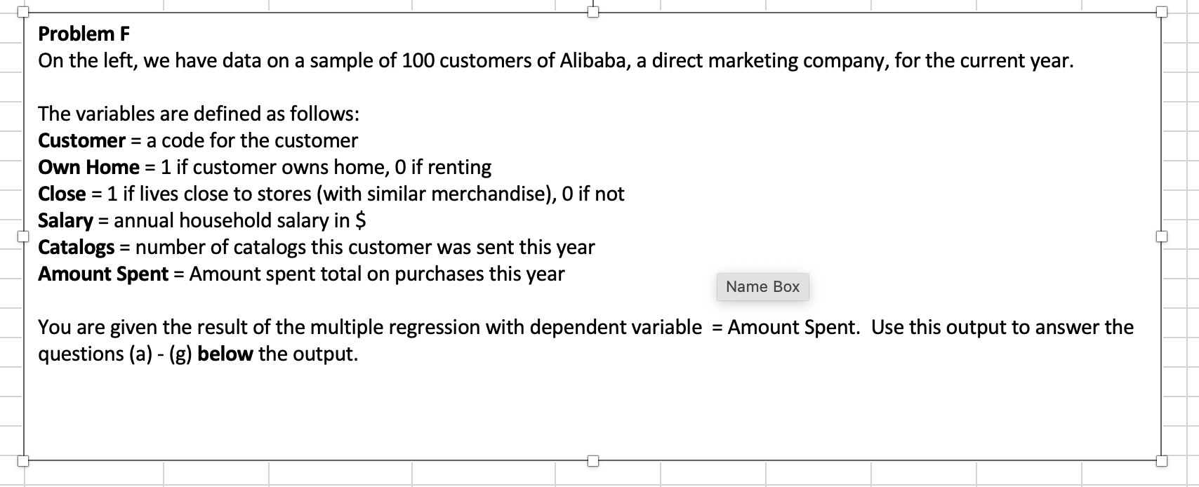
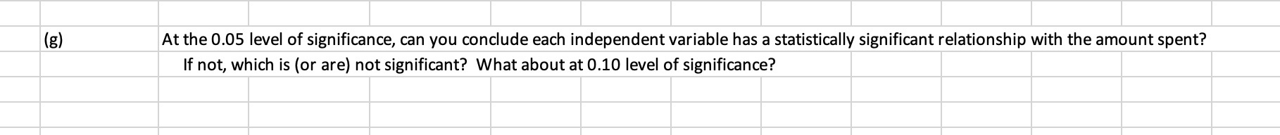
Problem F On the left, we have data on a sample of 100 customers of Alibaba, a direct marketing company, for the current year. The variables are defined as follows: Customer = a code for the customer Own Home =1 if customer owns home, 0 if renting Close =1 if lives close to stores (with similar merchandise), 0 if not Salary = annual household salary in $ Catalogs = number of catalogs this customer was sent this year Amount Spent = Amount spent total on purchases this year You are given the result of the multiple regression with dependent variable = Amount Spent. Use this output to answer the questions (a) - (g) below the output. (g) At the 0.05 level of significance, can you conclude each independent variable has a statistically significant relationship with the amount spent? If not, which is (or are) not significant? What about at 0.10 level of significance? \begin{tabular}{|c|c|c|c|c|c|c|} \hline \multicolumn{7}{|c|}{ SUMMARY OUTPUT } \\ \hline \multicolumn{7}{|c|}{ Regression Statistics } \\ \hline Multiple R & 0.8366 & & & & & \\ \hline R Square & 0.6999 & & & & & \\ \hline Adjusted R Squ & 0.6873 & & & & & \\ \hline Standard Error & 512.72 & & & & & \\ \hline Observations & 100 & & & & & \\ \hline \multicolumn{7}{|l|}{ ANOVA } \\ \hline & df & SS & MS & F & \multicolumn{2}{|l|}{ ignificance F} \\ \hline Regression & 4 & 58241400.88 & 14560350.22 & 55.39 & 0.000 & \\ \hline Residual & 95 & 24974011.87 & 262884.34 & & & \\ \hline Total & 99 & 83215412.75 & & & & \\ \hline & Coefficients & Standard Error & t Stat & P-value & Lower 95\% & Upper 95% \\ \hline Intercept & -91.67 & 185.917 & -0.493 & 0.623 & -460.76 & 277.42 \\ \hline Own Home & -229.47 & 121.800 & -1.884 & 0.063 & -471.27 & 12.34 \\ \hline Close & -604.90 & 114.229 & -5.295 & 0.000 & -831.67 & -378.12 \\ \hline Salary & 0.02216 & 0.002 & 9.836 & 0.000 & 0.02 & 0.03 \\ \hline Catalogs & 42.62 & 8.451 & 5.043 & 0.000 & 25.84 & 59.40 \\ \hline \end{tabular} Problem F On the left, we have data on a sample of 100 customers of Alibaba, a direct marketing company, for the current year. The variables are defined as follows: Customer = a code for the customer Own Home =1 if customer owns home, 0 if renting Close =1 if lives close to stores (with similar merchandise), 0 if not Salary = annual household salary in $ Catalogs = number of catalogs this customer was sent this year Amount Spent = Amount spent total on purchases this year You are given the result of the multiple regression with dependent variable = Amount Spent. Use this output to answer the questions (a) - (g) below the output. (g) At the 0.05 level of significance, can you conclude each independent variable has a statistically significant relationship with the amount spent? If not, which is (or are) not significant? What about at 0.10 level of significance? \begin{tabular}{|c|c|c|c|c|c|c|} \hline \multicolumn{7}{|c|}{ SUMMARY OUTPUT } \\ \hline \multicolumn{7}{|c|}{ Regression Statistics } \\ \hline Multiple R & 0.8366 & & & & & \\ \hline R Square & 0.6999 & & & & & \\ \hline Adjusted R Squ & 0.6873 & & & & & \\ \hline Standard Error & 512.72 & & & & & \\ \hline Observations & 100 & & & & & \\ \hline \multicolumn{7}{|l|}{ ANOVA } \\ \hline & df & SS & MS & F & \multicolumn{2}{|l|}{ ignificance F} \\ \hline Regression & 4 & 58241400.88 & 14560350.22 & 55.39 & 0.000 & \\ \hline Residual & 95 & 24974011.87 & 262884.34 & & & \\ \hline Total & 99 & 83215412.75 & & & & \\ \hline & Coefficients & Standard Error & t Stat & P-value & Lower 95\% & Upper 95% \\ \hline Intercept & -91.67 & 185.917 & -0.493 & 0.623 & -460.76 & 277.42 \\ \hline Own Home & -229.47 & 121.800 & -1.884 & 0.063 & -471.27 & 12.34 \\ \hline Close & -604.90 & 114.229 & -5.295 & 0.000 & -831.67 & -378.12 \\ \hline Salary & 0.02216 & 0.002 & 9.836 & 0.000 & 0.02 & 0.03 \\ \hline Catalogs & 42.62 & 8.451 & 5.043 & 0.000 & 25.84 & 59.40 \\ \hline \end{tabular}