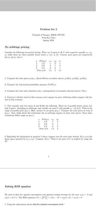
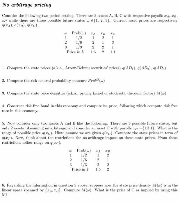
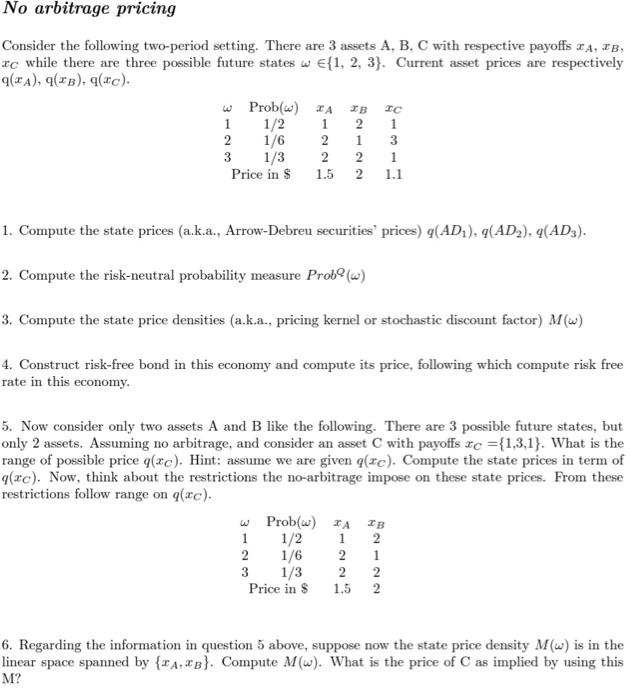
Problem Set 2 Spring, 2019 No arbitrage pricing e whike there are thove powible future states wE(1, 2.3 Cust prices are sespectively 1 1/2 2 1 2/6 23 3322 Price in $ 121 L Compute the state prkos (aka-Aman Debreu "curitav, prins) q(AD,)-gCADI, q(ADs). rabe in this ccoo range of pomide price (zc). Hid: aename wu are given 9(zr). Come the state prim in term of gre). Now,thiak about the restrictions the so-arbitge r on these stae prices From thes 11/212 21/6 2 3 13 2 limar spore sparand by {FA.rs). Cmpate M-), SI? t prawof C. implind by wa g thi. Soleing HJB equation No arbitrage pricing Consider the following two-period setting. There are 3 assets A, B, C with respective payoffs zA, B. rc while there are three possible future states w E1, 2, 3) Current asset prices are respectively q(xA), q(B), q(xc) 1 1/22 1 2 1/6 1 3 3 1/3 221 Price in 1.5 2 1.1 1. Compute the state prices (a.k.a., Arrow-Debreu securities' prices) (AD), q(AD2), q(AD3) 2. Compute the risk-neutral probability measure Prob (w) 3. Compute the state price densities (a.k.a., pricing kernel or stochastic discount factor) M(w) 4. Construct risk-free bond in this economy and compute its price, following which compute risk free rate in this economy 5. Now consider only two assets A and B like the following. There are 3 possible future states, but only 2 assets. Assuming no arbitrage, and consider an asset C with payoffs c 1,3,1. What is the range of possible price q(c). Hint: assume we are given q(xc) Compute the state prices in term of q(xc. Now, think about the restrictions the no-arbitrage impose on these state prices. From these restrictions follow range on q(rc) w Prob( A B 1 1/2 1 2 2 1/6 21 3 1/3 22 Price in S 1.5 2 6. Regarding the information in question 5 above, suppose now the state price density M( is in the linear space spanned by {xA,ZB), Compute M(w). what is the price of C as implied by using this M? No arbitrage pricing Consider the following two-period setting. There are 3 assets A, B, C with respective payoffs A, B, rc while there are three possible future states w E1, 2, 3). Current asset prices are respectively q(xA), q(B), q(xc) Prob A B c 1 1/221 2 1/6 2 3 3 1/3 221 Price in 1.5 2 1.1 1. Compute the state prices (a.k.a., Arrow-Debreu securities' prices) q(AD1), (AD2), (AD3) 2. Compute the risk-neutral probability measure Prob () 3. Compute the state price densities (a.k.a., pricing kernel or stochastic discount factor) M() 4. Construct risk-free bond in this economy and compute its price, following which compute risk free rate in this economy 5. Now consider only two assets A and B like the following. There are 3 possible future states, but only 2 assets. Assuming no arbitrage, and consider an asset C with payoffs rc 13,13. What is the range of possible price q(xc). Hint: assume we are given q(rc). Compute the state prices in term of q(c). Now, think about the restrictions the no-arbitrage impose on these state prices. From these restrictions follow range on q(rc) 1 1/2 2 2 1/621 3 1/3 2 Price in 1.5 2 6. Regarding the information in question 5 above, suppose now the state price density M(w) is in the linear space spanned by {xA,B. Compute M(). What is the price of C as implied by using this Problem Set 2 Spring, 2019 No arbitrage pricing e whike there are thove powible future states wE(1, 2.3 Cust prices are sespectively 1 1/2 2 1 2/6 23 3322 Price in $ 121 L Compute the state prkos (aka-Aman Debreu "curitav, prins) q(AD,)-gCADI, q(ADs). rabe in this ccoo range of pomide price (zc). Hid: aename wu are given 9(zr). Come the state prim in term of gre). Now,thiak about the restrictions the so-arbitge r on these stae prices From thes 11/212 21/6 2 3 13 2 limar spore sparand by {FA.rs). Cmpate M-), SI? t prawof C. implind by wa g thi. Soleing HJB equation No arbitrage pricing Consider the following two-period setting. There are 3 assets A, B, C with respective payoffs zA, B. rc while there are three possible future states w E1, 2, 3) Current asset prices are respectively q(xA), q(B), q(xc) 1 1/22 1 2 1/6 1 3 3 1/3 221 Price in 1.5 2 1.1 1. Compute the state prices (a.k.a., Arrow-Debreu securities' prices) (AD), q(AD2), q(AD3) 2. Compute the risk-neutral probability measure Prob (w) 3. Compute the state price densities (a.k.a., pricing kernel or stochastic discount factor) M(w) 4. Construct risk-free bond in this economy and compute its price, following which compute risk free rate in this economy 5. Now consider only two assets A and B like the following. There are 3 possible future states, but only 2 assets. Assuming no arbitrage, and consider an asset C with payoffs c 1,3,1. What is the range of possible price q(c). Hint: assume we are given q(xc) Compute the state prices in term of q(xc. Now, think about the restrictions the no-arbitrage impose on these state prices. From these restrictions follow range on q(rc) w Prob( A B 1 1/2 1 2 2 1/6 21 3 1/3 22 Price in S 1.5 2 6. Regarding the information in question 5 above, suppose now the state price density M( is in the linear space spanned by {xA,ZB), Compute M(w). what is the price of C as implied by using this M? No arbitrage pricing Consider the following two-period setting. There are 3 assets A, B, C with respective payoffs A, B, rc while there are three possible future states w E1, 2, 3). Current asset prices are respectively q(xA), q(B), q(xc) Prob A B c 1 1/221 2 1/6 2 3 3 1/3 221 Price in 1.5 2 1.1 1. Compute the state prices (a.k.a., Arrow-Debreu securities' prices) q(AD1), (AD2), (AD3) 2. Compute the risk-neutral probability measure Prob () 3. Compute the state price densities (a.k.a., pricing kernel or stochastic discount factor) M() 4. Construct risk-free bond in this economy and compute its price, following which compute risk free rate in this economy 5. Now consider only two assets A and B like the following. There are 3 possible future states, but only 2 assets. Assuming no arbitrage, and consider an asset C with payoffs rc 13,13. What is the range of possible price q(xc). Hint: assume we are given q(rc). Compute the state prices in term of q(c). Now, think about the restrictions the no-arbitrage impose on these state prices. From these restrictions follow range on q(rc) 1 1/2 2 2 1/621 3 1/3 2 Price in 1.5 2 6. Regarding the information in question 5 above, suppose now the state price density M(w) is in the linear space spanned by {xA,B. Compute M(). What is the price of C as implied by using this