

Question: Exploratory Data Analysis (No Answer Version). Make sure that you have completed ALL the exercises related to the lecture. Read the materials on tables from
Exploratory Data Analysis (No Answer Version).
Make sure that you have completed ALL the exercises related to the lecture.
Read the materials on tables from the following link:
https://support.office.com/en-us/article/Using-structured-references-with-Excel-tables-f5ed2452-2337-4f71-bed3-c8ae6d2b276e
- {using the Excel file Tables-Demo}
- Practice various calculations using the range without converting it into a table. Add the new record and then see if the average/sum of the sales in any of the area changes.
- Repeat the calculations but after converting the range to a table. What do you see now, when you insert the new data?
- Create a chart for the sales of the various region over the years.
- Create a way of capturing the range of the data (in years) in the chart title using COUNT and OFFSET function.
- {Using the Excel files Westside MLS Data Sept 05.xlsx and Credit Risk Data}
- Create frequency tables and histogram for the price in Westside MLS Data Sept 05.xlsx using the pivot table. Use the instructions in the word document that was uploaded. The bin size should be 100000.
- For the Credit Risk Data, using pivot table create frequency tables and histograms for the age of the customers using
- (a) 1-year bins starting at minimum age, (b) 5-year bins starting at age 15, (c) 10-year bins starting at age 10.
- Repeat the exercise in B and C above, but this time using the FREQUENCY function and following the instructions included in the word doc {HistogramstepsusingFreqfunction.docx}. Use 250000 as starting point for the real estate data and use a bin size of 100000. For the Credit Risk Data, use the same bin ranges and starting points as in part C above.
PS4 Exercise.
The Excel file PS4.xlsx (available on the Problem Set page) contains 4 worksheets with various types of data. 1 contains data on real estate listings, 2 contains data on credit risk of customers, 3 contains data on monthly stock price of Amazon, and 4 contains data on extended credit risk (from Camm et. al.). Using the file complete the following:
- Extract the unique Companies that list the various properties listed in Worksheet 1 using Advanced Filter available in Excel. How many unique companies are there?
- Using pivot table, develop a frequency table and a histogram for the Price column of the real estate data in Worksheet 1. Use a bin size of 100000. How many intervals are there if you include the intervals with no data (or zero frequency count)? Which range has the maximum number of observations and what is that number?
- Using pivot table, extract the Condo/Coop and Single Family Residential types of listing into two separate worksheets. For each one of them, create the frequency tables and corresponding histograms of price using pivot tables.
- Repeat task c, but this time using price/sqft as the measure instead of the price. How do the histograms differ? What conclusion can you make out of the two histograms?
- For the Single Family Residential listing that you extracted in part c above, create frequency chart and histogram but using FREQUENCY function and a bin size of 150000. What range contains the maximum number of observations and what is that number? [Hint: for this one, setup both the starting point as well as the bin size as cells so that you can easily change them. DO NOT FORGET THE CTRL+SHFT+ENTER part when entering the formula].
- The Worksheet 2 in PS4.xlsx contains the original data about credit risk for customers along with 3 new records that you have to insert in the range. Make a copy of this worksheet and using the data set in the copied worksheet and WITHOUT changing the range into a table,
- Calculate the average balance in the checking account for the customers in the original dataset (without the new records).
- Insert the three new records at the bottom of the original dataset. What is the balance in the checking account now? Did you have to do anything to update the balance?
- Create a column to the right of the dataset (column N) to calculate the combined balance customers have in their savings and the checking accounts. What is the average of the combined balance (after inclusion of the new records)?
- Make another copy of Worksheet 2. In this one, convert the original dataset to a Table and
- Calculate the average of the balance in the checking account.
- In column N for the first row of data (record number 1), build the formula for the combined balance by clicking on the corresponding cells for the checking account and savings account. What do you see once you hit Enter?
- Calculate the average of the combined balance.
- Insert the three new records provided at the bottom of the table, one at a time, and note the average balance for the checking account and the combined accounts after each insertion. Write down those values.
- For Worksheet 3,
- Change the graph in the Worksheet 3 to correctly reflect the months on the X-axis.
- Change the data area into a table so that insertion of new records are automatically included in the graph. Check it by inserting the stock price record for Jan-16 at the bottom of the original range.
- Currently, the title of the chart is static. Make it a dynamic title by creating text that should correctly include the range of the months used for the graph. Note that this range should come from the table with the data and should automatically update the BEGINNING MONTH and END MONTH based on the first row and the last row of the data. For example, if someone inserts the record for Feb-16 at the bottom and at the same time delete the record for Jan-15, then the graph title should automatically update to Amazon monthly stock price from Feb-15 to Feb-16. What functions did you have to use to make that happen?
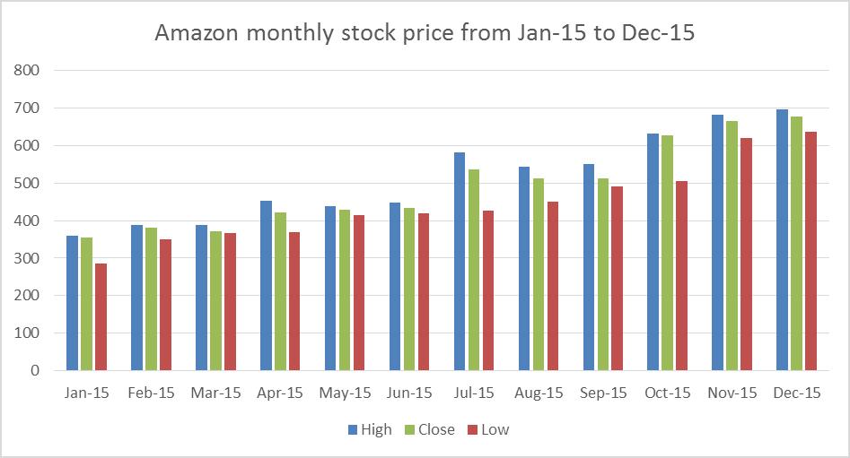
- Currently, the graph only includes the High and Close values for the stock price. Alter the graph to include the Low values as well. The resulting graph should look like the following:
- Create a formula in cell B2 of Worksheet 4 so that when a record number is entered in cell B1, the account number corresponding to that record number shows up WITHOUT ALTERING THE DATA at all. [Hint: OFFSET]
800 700 600 500 400 300 200 100 0 Amazon monthly stock price from Jan-15 to Dec-15 NO NO Jan-15 Feb-15 Mar-15 Apr-15 May-15 Jun-15 Jul-15 Aug-15 Sep-15 Oct-15 Nov-15 Dec-15 High I Close Low
Step by Step Solution
3.36 Rating (177 Votes )
There are 3 Steps involved in it
Here are the steps to respond to the queries using the content from the URL 1 Using structured references with Excel tables When you create an Excel table Excel assigns a name to the table and to each ... View full answer

Get step-by-step solutions from verified subject matter experts