Problem solutions must make full use of defined name ranges using the labels indicated for each Problem $5$: Charting

Re$-$create the Excel chart below $($Figure $7)$ that draws on the Forecasting worksheet data comparing the

total customer base under each of the two scenarios. Insert it at the top of the previous problem's

worksheet

Figure $7$: Market Capture Projections

There are multiple ways to create a chart like this. One way is to select the column of values for "Total

Customers" for the first scenario and create a simple chart.

Select the data and select: Insert $>$ Insert Line Chart $>($There are several chart types available;

you may use line or scatter chart type.$)$

Now from the second scenario select the values from the "Total Customers" column and copy

$($CTRL$-$C or Command$-$C$)$ to the system Clipboard.

Click the edge of the existing chart and paste $($CTRL$-$V or Command$-$V$)$ the Clipboard values to

add the second, comparison line.

You can click anywhere on the chart to reveal the three tool buttons beside the chart; use the

top tool $($or choose the option from the tool bar$)$ to modify various chart elements:

Chart Elements $,$ Chart Styles $,$ and Chart Filters

Or$,$ right$-$click on the specific area of the chart then select Format Chart Area options to refine

your chart elements with all appropriate labels, etc. as per the example

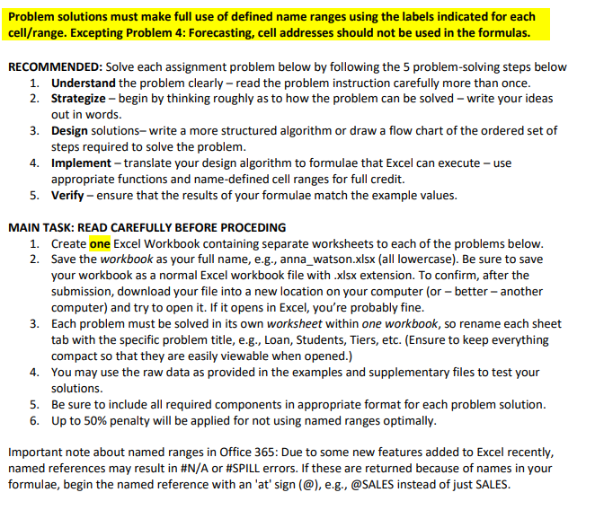
cell$/$range$.$ Excepting Problem $4$: Forecasting, cell addresses should not be used in the formulas.

RECOMMENDED: Solve each assignment problem below by following the $5$ problem$-$solving steps below

Understand the problem clearly $-$ read the problem instruction carefully more than once.

Strategize $-$ begin by thinking roughly as to how the problem can be solved $-$ write your ideas

out in words.

Design solutions$-$ write a more structured algorithm or draw a flow chart of the ordered set of

steps required to solve the problem.

Implement $-$ translate your design algorithm to formulae that Excel can execute $-$ use

appropriate functions and name$-$defined cell ranges for full credit.

Verify $-$ ensure that the results of your formulae match the example values.

MAIN TASK: READ CAREFULLY BEFORE PROCEDING

Create one Excel Workbook containing separate worksheets to each of the problems below.

Save the workbook as your full name, e$.$g$.,$ anna$\_$watson.xlsx $($all lowercase$).$ Be sure to save

your workbook as a normal Excel workbook file with $.$xlsx extension. To confirm, after the

submission, download your file into a new location on your computer $($or $-$ better $-$ another

computer$)$ and try to open it$.$ If it opens in Excel, you're probably fine.

Each problem must be solved in its own worksheet within one workbook, so rename each sheet

tab with the specific problem title, e$.$g$.,$ Loan, Students, Tiers, etc. $($Ensure to keep everything

compact so that they are easily viewable when opened.$)$

You may use the raw data as provided in the examples and supplementary files to test your

solutions.

Be sure to include all required components in appropriate format for each problem solution.

Up to $50\%$ penalty will be applied for not using named ranges optimally.

Important note about named ranges in Office $365$: Due to some new features added to Excel recently,

named references may result in #N$/$A or #SPILL errors. If these are returned because of names in your

formulae, begin the named reference with an $\text{'}$at$\text{'}$ sign $($@$),$ e$.$g$.,$ @SALES instead of just SALES.