Provide a short introduction to the problem. Describe the data: Perform and interpret the correlation analysis between all seven variables. Present and discuss the scatter diagram of Y against X1.

Estimate equation of the simple regression model Y = 0 + 1X1 + v (CW1.1) using Ordinary Least Squares method and interpret the magnitude and sign of the estimated coefficient 1. Assuming that the explanatory variable X1 in Equation (CW1.1) takes on average value, what is the point forecast of the Economic Rate of Return? What is the prediction interval? Provide an interpretation of the prediction interval

Estimate equation of a multiple regression model Y = 0 + 1X1 + 4X4 + 6X6 + u (CW1.2) using Ordinary Least Squares method. Present and interpret the estimates of the values of the parameters ( 0, 1, 4, and 6) and their estimated standard errors, the value of the residual sum of squares, and the R-Squared and Adjusted R-Squared.For each of the population parameters, 0, 1, 4, and 6, perform a test of the null hypothesis, H0 : j = 0, against the alternative hypothesis, H1 : j 6= 0, j = 0, 1, 4, 6. Also, perform the test of the joint hypothesis, H0 : 1 = 0, 4 = 0, 6 = 0, against the alternative hypothesis, H1 : 1 6= 0 or 4 6= 0 or 6 6= 0.Assume that the variance is unknown and the probability density function of the random disturbance term is normal. Provide economic interpretation of the testing

-The estimated coefficient at X1 becomes statistically insignificant in Equation CW1.2 compared to Equation CW1.1. Assess if this may be a result of multicollinearity in the model CW1.2. Discuss available remedies to tackle the problem of multicollinearity.

-Producing any additional evidence that is considered to be helpful, assess whether or not heteroskedasticity is a feature of the estimated model (Equation CW1.2). Discuss available remedies to tackle the problem of heteroskedasticity.

Briefly conclude

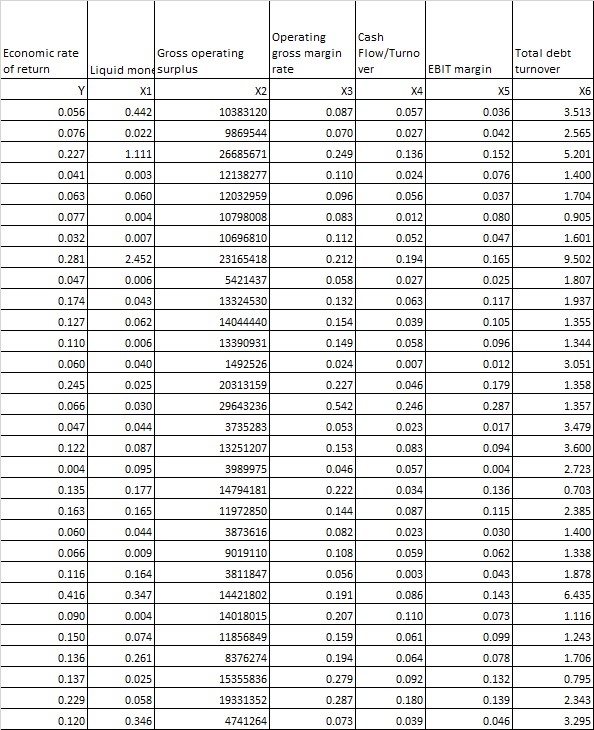
Operating Cash Economic rate Gross operating gross margin Flow/Turno Total debt of return Liquid monesurplus rate ver EBIT margin turnover Y X1 X2 X3 X6 0.056 0.442 10383120 0.087 0.057 0.036 3.513 0.076 0.027 9869544 0.070 0.027 0.042 2.565 0.227 1.111 26685671 0.249 0.136 0.152 5.201 0.041 0.003 12138277 0.110 0.024 0.076 1.400 0.06 D.060 12032959 0.096 0.056 0.037 1.704 0.077 0.004 10798008 0.083 0.012 0.080 0.90 0.032 0.007 10696810 0.112 0.052 0.047 1.601 0.281 2.452 23165418 0.212 0.194 0.165 9.50 0.047 0.006 6421437 0.058 0.027 0.025 1.80 0.174 0.043 13324530 0.132 0.063 0.117 1.937 0.127 0.062 14044440 0.154 0.039 0.105 1.35 0.110 0.006 0.149 0.058 0.096 1.34 0.060 0.040 1492526 0.024 0.007 0.012 3.051 0.245 0.025 20313159 0.227 0.046 0.179 1.358 0.066 0.030 29643236 0.542 0.246 0.287 1.357 0.047 0.044 3735283 0.053 0.023 0.017 3.479 0.122 0.087 13251207 0.153 0.083 0.09 3.60 0.004 0.09 1989975 0.046 0.057 0.004 2.72 0.135 0.177 14794181 0.222 0.034 0.136 0.703 0.165 0.165 11972850 0.144 0.087 0.115 2.385 0.060 0.044 3873616 0.082 0.02 0.030 1.40 0.06 0.009 9019110 0.108 0.059 0.062 1.338 0.116 0.164 3811847 0.056 0.003 0.043 1.878 0.416 0.347 14421802 0.191 0.086 D.143 5.43. 0.090 0.004 14018015 0.207 0.110 0.073 1.116 0.150 0.074 11856849 0.159 0.061 0.099 1.24 0.136 D.261 8376274 0.194 0.06 0.078 1.70 0.137 0.025 15355836 0.279 0.092 0.132 0.795 0.229 0.058 19331352 0.287 0.180 0.139 2.34 0.120 0.346 4741264 0.073 0.039 0.046 3.295