

Question: **Python Language can I get help? **bellow might help Programming Problem Modify your previous lab to do the following: 1. Using Python, work Ex 9.4
**Python Language can I get help?
**bellow might help
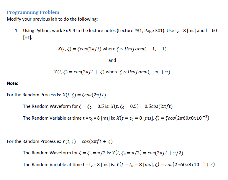
![8 [ms] and f = 60 [Hz]. X(t, 3) = {cos(2nft) where?](https://dsd5zvtm8ll6.cloudfront.net/si.experts.images/questions/2024/09/66f06bc33cedd_25866f06bc2c1820.jpg)
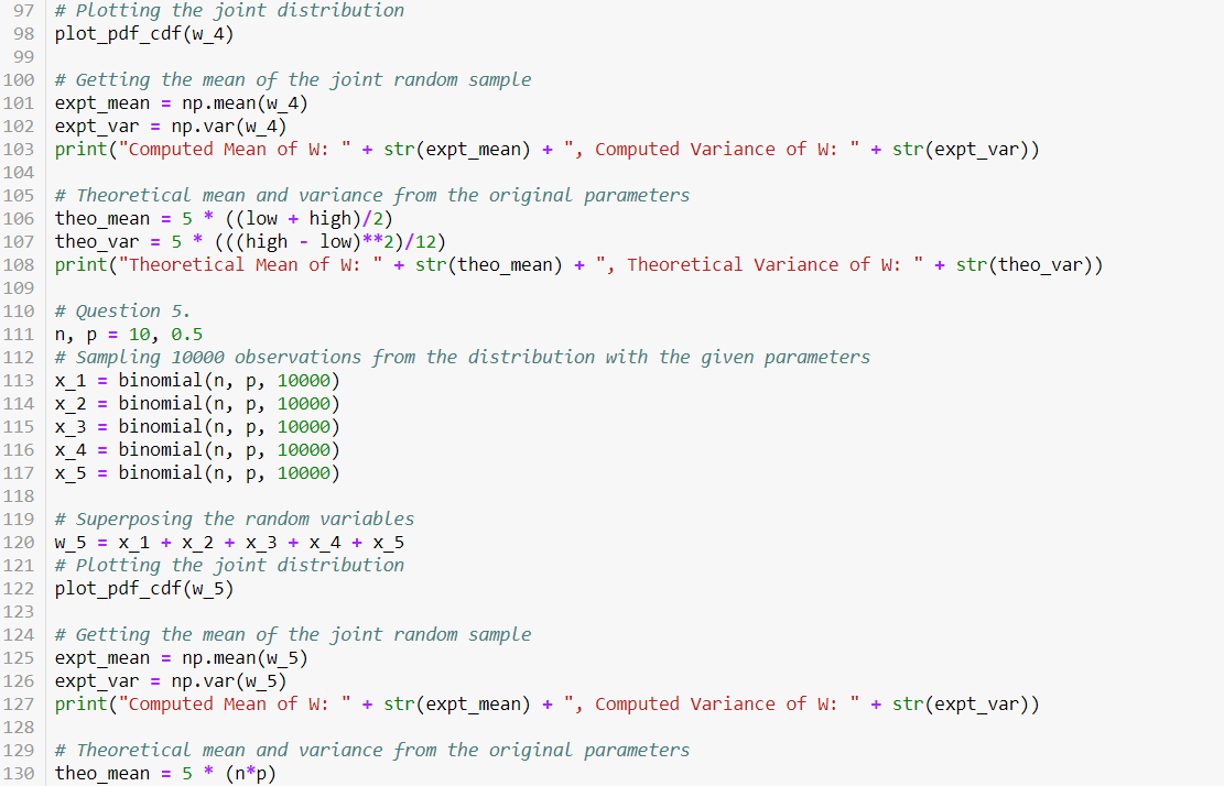
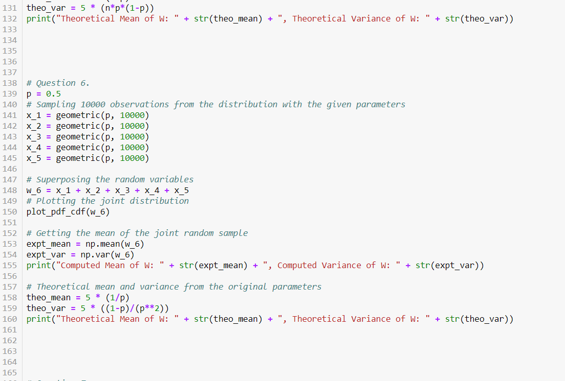
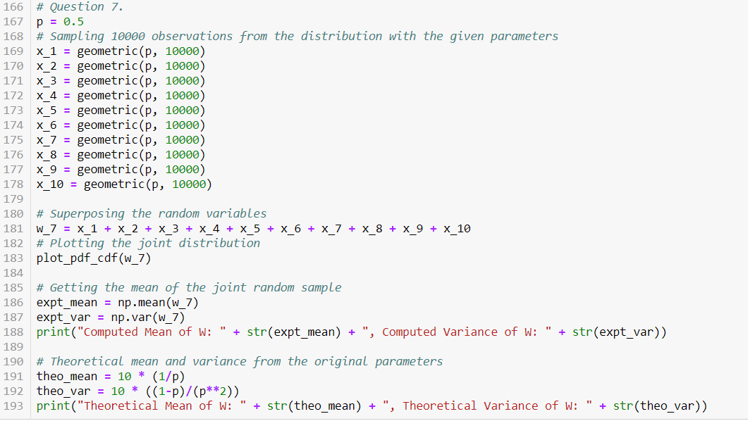
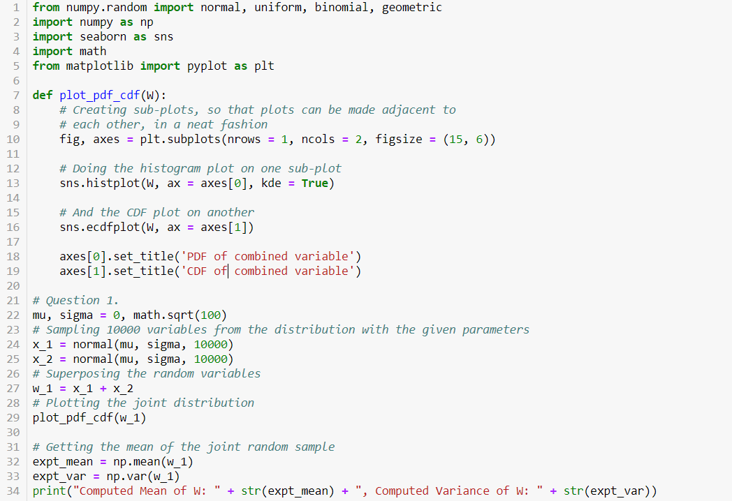
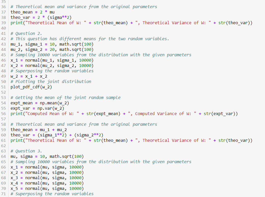
Programming Problem Modify your previous lab to do the following: 1. Using Python, work Ex 9.4 in the lecture notes (Lecture #31, Page 301). Use to = 8 [ms] and f = 60 [Hz]. X(t, 3) = {cos(2nft) where? Uniform( -1, + 1) and Y(t,5) = cos(2nft + ) where I ~ Uniform( - 1,+1) Note: For the Random Process is: X(t, 3) = {cos (2nft) The Random Waveform for 3 = 50 = 0.5 is: X(t, 50 = 0.5) = 0.5cos(2nft) The Random Variable at time t = to = 8 [ms] is: X(t = to = 8 [ms], 5) = {cos(2160x8x10-3) For the Random Process is: Y(t, 3) = cos(2nft + 3) The Random Waveform for 3 = 30 =/2 is: Y(t, 50 =1/2) = cos(2nft +n/2) The Random Variable at time t = to = 8 [ms] is: Y(t = to = 8 [ms], 5) = cos(2160x8x10-3+5) 5 8 9 10 1 from numpy.random import normal, uniform, binomial, geometric 2 import numpy as np 3 import seaborn as sns 4 import math from matplotlib import pyplot as plt 6 7 def plot_pdf_cdf(w): # Creating sub-plots, so that plots can be made adjacent to # each other, in a neat fashion fig, axes = plt.subplots(nrows = 1, ncols = 2, figsize = (15, 6)) 11 12 # Doing the histogram plot on one sub-plot 13 sns.histplot(W, ax = axes[0], kde = True) 14 15 # And the CDF plot on another 16 sns.ecdfplot(W, ax = axes[1]) 17 18 axes[0].set_title('PDF of combined variable') 19 axes[1].set_title('CDF of combined variable') 20 21 # Question 1. 22 mu, sigma = 0, math.sqrt(100) 23 # Sampling 10000 variables from the distribution with the given parameters 24 x_1 = normal (mu, sigma, 10000) 25 x_2 = normal(mu, sigma, 10000) 26 # Superposing the random variables 27 W_1 = x_1 + X_2 28 # Plotting the joint distribution 29 plot_pdf_cdf(w_1) 30 31 # Getting the mean of the joint random sample 32 expt_mean = np.mean(w_1) 33 expt_var = np.var(w_1) 34 print("Computed Mean of W: " + str(expt_mean) ', Computed Variance of W: + + str(expt_var)) 35 36 # Theoretical mean and variance from the original parameters 37 theo_mean = 2 * mu 38 theo_var = 2 * (sigma**2) 39 print("Theoretical Mean of W: " + str(theo_mean) + ". ", Theoretical Variance of W: " + str(theo_var)) 40 41 # Question 2. 42 # This question has different means for the two random variables. 43 mu_1, sigma_1 = 10, math.sqrt(100) 44 mu_2, sigma_2 = 20, math.sqrt(100) 45 # Sampling 10000 variables from the distribution with the given parameters x_1 = normal (mu_1, sigma_1, 10000) 47 X_2 = normal (mu_2, sigma_2, 10000) # Superposing the random variables 49 W_2 = X_1 + X_2 50 # Plotting the joint distribution 51 plot_pdf_cdf(w_2) 46 48 52 + 61 53 # Getting the mean of the joint random sample 54 expt_mean = np.mean(w_2) 55 expt_var = np.var(w_2) 56 print("Computed Mean of W: " + str(expt_mean) + ", Computed Variance of W: " + str(expt_var)) 57 58 # Theoretical mean and variance from the original parameters 59 theo_mean = mu_1 + mu_2 60 theo_var = (sigma_1**2) (sigma_2**2) print("Theoretical Mean of W: " + str(theo_mean) + ", Theoretical Variance of W: + str(theo_var)) 62 # Question 3. 64 mu, sigma = 10, math.sqrt(100) # Sampling 10000 variables from the distribution with the given parameters X_1 = normal(mu, sigma, 10000) x_2 = normal(mu, sigma, 10000) X_3 = normal (mu, sigma, 10000) 69 x_4 = normal(mu, sigma, 10000) 70 x_5 = normal (mu, sigma, 10000) # Superposing the random variables 63 65 66 67 68 71 71 82 # Superposing the random Variables 72 W_3 = x_1 + x_2 + x_3 + X_4 + x_5 73 # Plotting the joint distribution 74 plot_pdf_cdf(w_3) 75 76 # Getting the mean of the joint random sample 77 expt_mean = np.mean(w_3) 78 expt_var = np.var(w_3) 79 print("Computed Mean of W: " + str(expt_mean) + ", Computed Variance of W: + str(expt_var)) 80 81 # Theoretical mean and variance from the original parameters theo mean = 5 * mu 83 theo_var = 5 * (sigma**2) 84 print("Theoretical Mean of W: " + str(theo_mean) + ", Theoretical Variance of w: + str(theo_var)) 85 86 # Question 4. 87 low, high = 0, 10 88 # Sampling 10000 observations from the distribution with the given parameters 89 x_1 = uniform(low, high, 10000) 90 x_2 = uniform(low, high, 10000) 91 x_3 = uniform(low, high, 10000) 92 x_4 = uniform(low, high, 10000) 93 x 5 = uniform(low, high, 10000) 94 95 # Superposing the random variables 96 W_4 = x_1 + X_2 + X_3 + X_4 + X_5 97 # Plotting the joint distribution 98 plot_pdf_cdf(w_4) 99 00 # Getting the mean of the joint random sample 01 expt_mean = np.mean(w_4) 02 expt_var = np.var(w_4) 03 print("Computed Mean of W: " + str(expt_mean) + ", Computed Variance of W: + str(expt_var)) 04 05 # Theoretical mean and variance from the original parameters theo mean = 5 * ((low + high)/2) " 06 97 # Plotting the joint distribution 98 plot_pdf_cdf(w_4) 99 100 # Getting the mean of the joint random sample 101 expt_mean = np.mean(w_4) 102 expt_var = np.var(w_4) 103 print("Computed Mean of W: " + str(expt_mean) + ", Computed Variance of W: " + str(expt_var)) 104 105 # Theoretical mean and variance from the original parameters 106 theo_mean = 5 * ((low + high)/2) 107 theo_var = 5 * (((high - low)**2)/12) 108 print("Theoretical Mean of W: " + str(theo_mean) + ", Theoretical Variance of W: " + str(theo_var)) 109 110 # Question 5. n, p = 10, 0.5 112 # Sampling 10000 observations from the distribution with the given parameters 113 x_1 = binomial(n, p, 10000) 114 x_2 = binomial(n, p, 10000) 115 x_3 = binomial(n, p, 10000) 116 x_4 = binomial(n, p, 10000) 117 x_5 = binomial(n, p, 10000) 118 119 # Superposing the random variables 120 w_5 = x_1 + X_2 + x_3 + x_4 + x_5 121 # Plotting the joint distribution 122 plot_pdf_cdf(w_5) 111 123 11 124 # Getting the mean of the joint random sample 125 expt_mean = np.mean(w_5) 126 expt_var = np.var(w_5) 127 print("Computed Mean of W: + str(expt_mean) + ", Computed Variance of W: " 128 129 # Theoretical mean and variance from the original parameters 130 theo mean = 5 * (n*p) + str(expt_var)) 131 theo_var = 5 * (n*p*(1-P)) 132 print("Theoretical Mean of w: + str(theo_mean) + ", Theoretical Variance of W: + str(theo_var)) 133 134 135 136 137 138 # Question 6. 139 p = 0.5 140 # Sampling 10000 observations from the distribution with the given parameters 141 x_1 = geometric(p, 10000) 142 x_2 = geometric(p, 10000) 143 x_3 = geometric(p, 10000) 144 x_4 = geometric(p, 10000) 145 x_5 = geometric(p, 10000) 146 147 # Superposing the random variables 148 W_6 = X_1 + X_2 + x_3 + x_4 + x_5 149 # Plotting the joint distribution 150 plot_pdf_cdf(w_6) 151 152 # Getting the mean of the joint random sample 153 expt_mean = np.mean(w_6) 154 expt_var = np.var(w_6) 155 print("Computed Mean of w: + str(expt_mean) + ", Computed Variance of W: + str(expt_var)) 156 157 # Theoretical mean and variance from the original parameters 158 theo_mean = 5 * (1/p) 159 theo_var = 5 * ((1-p)/(p**2)) 160 print("Theoretical Mean of W: + str(theo_mean) + ", Theoretical Variance of W: + str(theo_var)) 161 162 163 164 165 166 # Question 7. 167 p = 0.5 168 # Sampling 10000 observations from the distribution with the given parameters 169 x_1 = geometric(p, 10000) 170 x_2 = geometric(p, 10000) 171 x_3 = geometric(p, 10000) 172 x_4 = geometric(p, 10000) 173 x_5 = geometric(p, 10000) 174 x 6 = geometric(p, 10000) 175 x_7 = geometric(p, 10000) 176 x 8 = geometric(p, 10000) 177 x_9 = geometric(p, 10000) 178 X_10 = geometric(p, 10000) 179 180 # Superposing the random variables 181 W_7 = X_1 + X_2 + x_3 + x_4 + x_5 + X_6 + X_7 + X_8 + X_9 + X_10 182 # plotting the joint distribution 183 plot_pdf_cdf(w_7) 184 185 # Getting the mean of the joint random sample 186 expt_mean = np.mean(w_7) 187 expt_var = np.var(w_7) 188 print("Computed Mean of W: + str(expt_mean) + ", Computed Variance of W: + str(expt_var)) 189 190 # Theoretical mean and variance from the original parameters 191 theo_mean = 10 * (1/p) 192 theo_var = 10 * ((1-p)/(p**2)) 193 print("Theoretical Mean of w: + str(theo_mean) Theoretical Variance of W: + str(theo_var)) + Programming Problem Modify your previous lab to do the following: 1. Using Python, work Ex 9.4 in the lecture notes (Lecture #31, Page 301). Use to = 8 [ms] and f = 60 [Hz]. X(t, 3) = {cos(2nft) where? Uniform( -1, + 1) and Y(t,5) = cos(2nft + ) where I ~ Uniform( - 1,+1) Note: For the Random Process is: X(t, 3) = {cos (2nft) The Random Waveform for 3 = 50 = 0.5 is: X(t, 50 = 0.5) = 0.5cos(2nft) The Random Variable at time t = to = 8 [ms] is: X(t = to = 8 [ms], 5) = {cos(2160x8x10-3) For the Random Process is: Y(t, 3) = cos(2nft + 3) The Random Waveform for 3 = 30 =/2 is: Y(t, 50 =1/2) = cos(2nft +n/2) The Random Variable at time t = to = 8 [ms] is: Y(t = to = 8 [ms], 5) = cos(2160x8x10-3+5) 5 8 9 10 1 from numpy.random import normal, uniform, binomial, geometric 2 import numpy as np 3 import seaborn as sns 4 import math from matplotlib import pyplot as plt 6 7 def plot_pdf_cdf(w): # Creating sub-plots, so that plots can be made adjacent to # each other, in a neat fashion fig, axes = plt.subplots(nrows = 1, ncols = 2, figsize = (15, 6)) 11 12 # Doing the histogram plot on one sub-plot 13 sns.histplot(W, ax = axes[0], kde = True) 14 15 # And the CDF plot on another 16 sns.ecdfplot(W, ax = axes[1]) 17 18 axes[0].set_title('PDF of combined variable') 19 axes[1].set_title('CDF of combined variable') 20 21 # Question 1. 22 mu, sigma = 0, math.sqrt(100) 23 # Sampling 10000 variables from the distribution with the given parameters 24 x_1 = normal (mu, sigma, 10000) 25 x_2 = normal(mu, sigma, 10000) 26 # Superposing the random variables 27 W_1 = x_1 + X_2 28 # Plotting the joint distribution 29 plot_pdf_cdf(w_1) 30 31 # Getting the mean of the joint random sample 32 expt_mean = np.mean(w_1) 33 expt_var = np.var(w_1) 34 print("Computed Mean of W: " + str(expt_mean) ', Computed Variance of W: + + str(expt_var)) 35 36 # Theoretical mean and variance from the original parameters 37 theo_mean = 2 * mu 38 theo_var = 2 * (sigma**2) 39 print("Theoretical Mean of W: " + str(theo_mean) + ". ", Theoretical Variance of W: " + str(theo_var)) 40 41 # Question 2. 42 # This question has different means for the two random variables. 43 mu_1, sigma_1 = 10, math.sqrt(100) 44 mu_2, sigma_2 = 20, math.sqrt(100) 45 # Sampling 10000 variables from the distribution with the given parameters x_1 = normal (mu_1, sigma_1, 10000) 47 X_2 = normal (mu_2, sigma_2, 10000) # Superposing the random variables 49 W_2 = X_1 + X_2 50 # Plotting the joint distribution 51 plot_pdf_cdf(w_2) 46 48 52 + 61 53 # Getting the mean of the joint random sample 54 expt_mean = np.mean(w_2) 55 expt_var = np.var(w_2) 56 print("Computed Mean of W: " + str(expt_mean) + ", Computed Variance of W: " + str(expt_var)) 57 58 # Theoretical mean and variance from the original parameters 59 theo_mean = mu_1 + mu_2 60 theo_var = (sigma_1**2) (sigma_2**2) print("Theoretical Mean of W: " + str(theo_mean) + ", Theoretical Variance of W: + str(theo_var)) 62 # Question 3. 64 mu, sigma = 10, math.sqrt(100) # Sampling 10000 variables from the distribution with the given parameters X_1 = normal(mu, sigma, 10000) x_2 = normal(mu, sigma, 10000) X_3 = normal (mu, sigma, 10000) 69 x_4 = normal(mu, sigma, 10000) 70 x_5 = normal (mu, sigma, 10000) # Superposing the random variables 63 65 66 67 68 71 71 82 # Superposing the random Variables 72 W_3 = x_1 + x_2 + x_3 + X_4 + x_5 73 # Plotting the joint distribution 74 plot_pdf_cdf(w_3) 75 76 # Getting the mean of the joint random sample 77 expt_mean = np.mean(w_3) 78 expt_var = np.var(w_3) 79 print("Computed Mean of W: " + str(expt_mean) + ", Computed Variance of W: + str(expt_var)) 80 81 # Theoretical mean and variance from the original parameters theo mean = 5 * mu 83 theo_var = 5 * (sigma**2) 84 print("Theoretical Mean of W: " + str(theo_mean) + ", Theoretical Variance of w: + str(theo_var)) 85 86 # Question 4. 87 low, high = 0, 10 88 # Sampling 10000 observations from the distribution with the given parameters 89 x_1 = uniform(low, high, 10000) 90 x_2 = uniform(low, high, 10000) 91 x_3 = uniform(low, high, 10000) 92 x_4 = uniform(low, high, 10000) 93 x 5 = uniform(low, high, 10000) 94 95 # Superposing the random variables 96 W_4 = x_1 + X_2 + X_3 + X_4 + X_5 97 # Plotting the joint distribution 98 plot_pdf_cdf(w_4) 99 00 # Getting the mean of the joint random sample 01 expt_mean = np.mean(w_4) 02 expt_var = np.var(w_4) 03 print("Computed Mean of W: " + str(expt_mean) + ", Computed Variance of W: + str(expt_var)) 04 05 # Theoretical mean and variance from the original parameters theo mean = 5 * ((low + high)/2) " 06 97 # Plotting the joint distribution 98 plot_pdf_cdf(w_4) 99 100 # Getting the mean of the joint random sample 101 expt_mean = np.mean(w_4) 102 expt_var = np.var(w_4) 103 print("Computed Mean of W: " + str(expt_mean) + ", Computed Variance of W: " + str(expt_var)) 104 105 # Theoretical mean and variance from the original parameters 106 theo_mean = 5 * ((low + high)/2) 107 theo_var = 5 * (((high - low)**2)/12) 108 print("Theoretical Mean of W: " + str(theo_mean) + ", Theoretical Variance of W: " + str(theo_var)) 109 110 # Question 5. n, p = 10, 0.5 112 # Sampling 10000 observations from the distribution with the given parameters 113 x_1 = binomial(n, p, 10000) 114 x_2 = binomial(n, p, 10000) 115 x_3 = binomial(n, p, 10000) 116 x_4 = binomial(n, p, 10000) 117 x_5 = binomial(n, p, 10000) 118 119 # Superposing the random variables 120 w_5 = x_1 + X_2 + x_3 + x_4 + x_5 121 # Plotting the joint distribution 122 plot_pdf_cdf(w_5) 111 123 11 124 # Getting the mean of the joint random sample 125 expt_mean = np.mean(w_5) 126 expt_var = np.var(w_5) 127 print("Computed Mean of W: + str(expt_mean) + ", Computed Variance of W: " 128 129 # Theoretical mean and variance from the original parameters 130 theo mean = 5 * (n*p) + str(expt_var)) 131 theo_var = 5 * (n*p*(1-P)) 132 print("Theoretical Mean of w: + str(theo_mean) + ", Theoretical Variance of W: + str(theo_var)) 133 134 135 136 137 138 # Question 6. 139 p = 0.5 140 # Sampling 10000 observations from the distribution with the given parameters 141 x_1 = geometric(p, 10000) 142 x_2 = geometric(p, 10000) 143 x_3 = geometric(p, 10000) 144 x_4 = geometric(p, 10000) 145 x_5 = geometric(p, 10000) 146 147 # Superposing the random variables 148 W_6 = X_1 + X_2 + x_3 + x_4 + x_5 149 # Plotting the joint distribution 150 plot_pdf_cdf(w_6) 151 152 # Getting the mean of the joint random sample 153 expt_mean = np.mean(w_6) 154 expt_var = np.var(w_6) 155 print("Computed Mean of w: + str(expt_mean) + ", Computed Variance of W: + str(expt_var)) 156 157 # Theoretical mean and variance from the original parameters 158 theo_mean = 5 * (1/p) 159 theo_var = 5 * ((1-p)/(p**2)) 160 print("Theoretical Mean of W: + str(theo_mean) + ", Theoretical Variance of W: + str(theo_var)) 161 162 163 164 165 166 # Question 7. 167 p = 0.5 168 # Sampling 10000 observations from the distribution with the given parameters 169 x_1 = geometric(p, 10000) 170 x_2 = geometric(p, 10000) 171 x_3 = geometric(p, 10000) 172 x_4 = geometric(p, 10000) 173 x_5 = geometric(p, 10000) 174 x 6 = geometric(p, 10000) 175 x_7 = geometric(p, 10000) 176 x 8 = geometric(p, 10000) 177 x_9 = geometric(p, 10000) 178 X_10 = geometric(p, 10000) 179 180 # Superposing the random variables 181 W_7 = X_1 + X_2 + x_3 + x_4 + x_5 + X_6 + X_7 + X_8 + X_9 + X_10 182 # plotting the joint distribution 183 plot_pdf_cdf(w_7) 184 185 # Getting the mean of the joint random sample 186 expt_mean = np.mean(w_7) 187 expt_var = np.var(w_7) 188 print("Computed Mean of W: + str(expt_mean) + ", Computed Variance of W: + str(expt_var)) 189 190 # Theoretical mean and variance from the original parameters 191 theo_mean = 10 * (1/p) 192 theo_var = 10 * ((1-p)/(p**2)) 193 print("Theoretical Mean of w: + str(theo_mean) Theoretical Variance of W: + str(theo_var)) +
Step by Step Solution
There are 3 Steps involved in it

Get step-by-step solutions from verified subject matter experts