Python language please. Thank you!

#%% md

# Setup

First, let's import a few common modules, ensure MatplotLib plots figures inline and prepare a function to save the figures. We also check that Python 3.5 or later is installed (although Python 2.x may work, it is deprecated so we strongly recommend you use Python 3 instead), as well as Scikit-Learn 0.20.

#%%

# Python 3.5 is required

import sys

assert sys.version_info >= (3, 5)

# Scikit-Learn 0.20 is required

import sklearn

assert sklearn.__version__ >= "0.20"

# Common imports

import numpy as np

import os

# to make this notebook's output stable across runs

np.random.seed(42)

# To plot pretty figures

%matplotlib inline

import matplotlib as mpl

import matplotlib.pyplot as plt

mpl.rc('axes', labelsize=14)

mpl.rc('xtick', labelsize=12)

mpl.rc('ytick', labelsize=12)

# Where to save the figures

PROJECT_ROOT_DIR = "."

CHAPTER_ID = "training_linear_models"

IMAGES_PATH = os.path.join(PROJECT_ROOT_DIR, "images", CHAPTER_ID)

os.makedirs(IMAGES_PATH, exist_ok=True)

def save_fig(fig_id, tight_layout=True, fig_extension="png", resolution=300):

path = os.path.join(IMAGES_PATH, fig_id + "." + fig_extension)

print("Saving figure", fig_id)

if tight_layout:

plt.tight_layout()

plt.savefig(path, format=fig_extension, dpi=resolution)

# Ignore useless warnings (see SciPy issue #5998)

import warnings

warnings.filterwarnings(action="ignore", message="^internal gelsd")

#%% md

# Linear regression using the Normal Equation

#%%

import numpy as np

X = 2 * np.random.rand(100, 1)

y = 4 + 3 * X + np.random.randn(100, 1)

#%%

plt.plot(X, y, "b.")

plt.xlabel("$x_1$", fontsize=18)

plt.ylabel("$y$", rotation=0, fontsize=18)

plt.axis([0, 2, 0, 15])

save_fig("generated_data_plot")

plt.show()

#%%

X_b = np.c_[np.ones((100, 1)), X] # add x0 = 1 to each instance

theta_best = np.linalg.inv(X_b.T.dot(X_b)).dot(X_b.T).dot(y)

#%%

theta_best

#%%

X_new = np.array([[0], [2]])

X_new_b = np.c_[np.ones((2, 1)), X_new] # add x0 = 1 to each instance

y_predict = X_new_b.dot(theta_best)

y_predict

#%%

plt.plot(X_new, y_predict, "r-")

plt.plot(X, y, "b.")

plt.axis([0, 2, 0, 15])

plt.show()

#%% md

adding labels and legend to the plot

#%%

plt.plot(X_new, y_predict, "r-", linewidth=2, label="Predictions")

plt.plot(X, y, "b.")

plt.xlabel("$x_1$", fontsize=18)

plt.ylabel("$y$", rotation=0, fontsize=18)

plt.legend(loc="upper left", fontsize=14)

plt.axis([0, 2, 0, 15])

save_fig("linear_model_predictions_plot")

plt.show()

#%% md

# sklearn models

#%%

from sklearn.linear_model import LinearRegression

lin_reg = LinearRegression()

lin_reg.fit(X, y)

lin_reg.intercept_, lin_reg.coef_

#%%

lin_reg.predict(X_new)

#%% md

The LinearRegression class is based on the scipy.linalg.lstsq() function (the name stands for "least squares"), which you could call directly:

#%%

theta_best_svd, residuals, rank, s = np.linalg.lstsq(X_b, y, rcond=1e-6)

theta_best_svd

#%% md

This function computes $\mathbf{X}^+\mathbf{y}$, where $\mathbf{X}^{+}$ is the pseudoinverse of $\mathbf{X}$ (specifically the Moore-Penrose inverse). You can use np.linalg.pinv() to compute the pseudoinverse directly:

#%% md

# Linear regression using batch gradient descent

#%% md

# a

[6 Marks]

Write a simple implementation of a least-squares solution to linear regression that applies an iterative update to adjust the weights. Demonstrate the success of your approach on the sample data loaded below, and visualize the best fit plotted as a line (consider using linspace) against a scatter plot of the x and y test values

#%%

##### YOUR CODE HERE #######

#%% md

# b

[6 Marks]

Load data on movie ratings, revenue, metadata etc. Split data into a relevant set for training, testing and classification. Explain your choice of split. It is ok if you decide to split into these subsets after part c -> if you do so, mention this at the end of your explanation.

Explanation:

#%%

### An example to load a csv file

import pandas as pd

import numpy as np

from ast import literal_eval

meta_data=pd.read_csv('movies_metadata.csv', low_memory=False) # You may wish to specify types, or process columns once read

ratings_small=pd.read_csv('ratings_small.csv')

import warnings; warnings.simplefilter('ignore')

##### YOUR CODE HERE #######

#%%

#%% md

# c

[6 Marks]

#%% md

Organize the data into relevant features for predicting revenue.

i. Explain your feature sets and organization.

YOUR EXPLANATION HERE

ii. Plot movie revenue vs. rating as a scatter plot and discuss your findings.

YOUR EXPLANATION HERE

iii. Visualize any other relationships you deem interesting and explain.

YOUR EXPLANATION HERE

#%%

meta_data.head(10)

# The following line is one way of cleaning up the genres field - there are more verbose ways of doing this that are easier for a human to read

#meta_data['genres'] = meta_data['genres'].fillna('[]').apply(literal_eval).apply(lambda x: [i['name'] for i in x] if isinstance(x, list) else [])

#meta_data['year'] = pd.to_datetime(meta_data['release_date'], errors='coerce').apply(lambda x: str(x).split('-')[0] if x != np.nan else np.nan)

meta_data.head()

# Consider how to columns look before and after this 'clean-up' - it is very common to have to massage the data to get the right features

#ratings_small.head()

##### YOUR CODE HERE #######

Here are screenshots of what the code looks like:

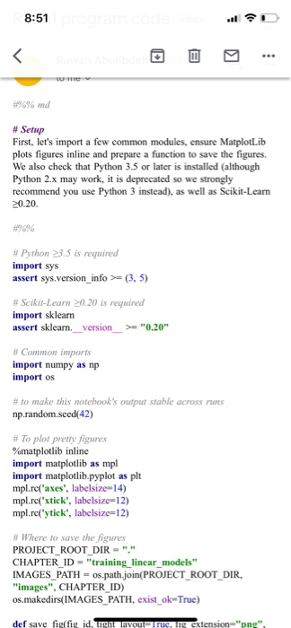
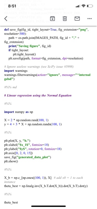
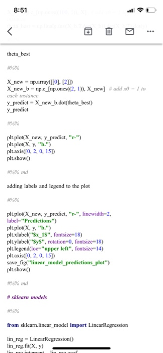
provided. Details of what steps are required are included in the Jupyter notebook itself. Summary of Programming part I elements (Detailed requirements are in the notebook markdown itself) 1. Simple implementation of incremental least squares (from scratch) (5 points) 2. Reading in data related to movies, split into train, validation, test. (5 points) 3. Developing features, understanding properties of the data, visualization. (5 points) 8:51 Tv #%% md # Setup First, let's import a few common modules, ensure MatplotLib plots figures inline and prepare a function to save the figures. We also check that Python 3.5 or later is installed (although Python 2.x may work, it is deprecated so we strongly recommend you use Python 3 instead), as well as Scikit-Learn 20.20. #9% # Python 3.5 is required import sys assert sys.version_info > (3,5) # Scikit-Learn 0.20 is required import sklearn assert sklearn._version >= "0.20" # Common imports import numpy as np import os # to make this notebook's output stable across np.random.seed(42) # To plor pretty figures %matplotlib inline import matplotlib as mpl import matplotlib.pyplot as plt mpl.re('axes', labelsize=14) mpi.re('xtick', labelsize=12) mpl.re('ytick', labelsize=12) # Where to save the figures PROJECT_ROOT_DIR="." CHAPTER_ID = "training linear_models" IMAGES_PATH = os.path.join(PROJECT_ROOT_DIR, "images", CHAPTER ID) os.makedirs(IMAGES_PATH, exist_ok-True) def save fig(fig id, tight avou F1 rue, g extension="png", 8:51 def save_fig(fig_id, tight_layout=True, fig_extension="png", resolution=300): path = os.path.join(IMAGES_PATH, fig_id + "." + fig extension) print("Saving figure", fig_id) if tight_layout: plt.tight_layout() plt.savefig(path, format=fig_extension, dpi-resolution) #Ignore useless warnings (see Scipy issue #5998) import warnings warnings.filterwarnings action="ignore", message="internal gelsd") #%% md # Linear regression using the Normal Equation import numpy as np X-2* np.random.rand(100, 1) y = 4 + 3 * X + np.random.randn(100, 1) plt.plot(x, y, ".") plt.xlabel("Sx_15", fontsize=18) plt.ylabel("Sys", rotation=0, fontsize=18) plt.axis([0, 2, 0, 151) save_fig("generated_data_plot") plt.show X_ b np.c_[np.ones (100, 1)), X] #add x0 = to each instance theta_best = np.linalg.inv(X_b.T.dot(X_b)).dot(X_b.T).dot(y) theta_best 8:51 theta best X_new = np.array([[0], [21]) X_new_b - np.c_(np.ones((2,1)), X_new] # add x0 = 1 to each instance y predict X_new_b.dot(theta_best) y predict #%% plt.plot(X new, y predict, "r.") plt.plot(x, y, ".") plt.axis([0, 2, 0, 15]) plt.show() #%% md adding labels and legend to the plot %% plt.plot(X_new, y predict, "r-", linewidth-2, label="Predictions") plt.plot(x, y, "b.") plt.xlabel("$x_15", fontsize=18) plt.ylabel("Sys", rotation-0, fontsize=18) plt.legend(loc"upper left", fontsize=14) plt.axis([0, 2, 0, 151) save_fig("linear_model_predictions_plot") plt.show #%% md # sklearn models from sklearn.linear model import LincarRegression lin_reg - LinearRegression lin_reg.fit(x, y) 8:51 # sklearn models from sklearn.linear_model import Linear Regression lin reg = LinearRegression lin reg.fit(x, y) lin_reg. intercept, lin_reg.coef lin_reg.predict(X_new) #%% md The Linear Regression class is based on the scipy.linalg. Istsqo function (the name stands for "least squares"), which you could call directly theta_best_svd, residuals, rank, s = np.linalg.Istsq(X_b, y, rcond=le-6) theta best svd #%% md This function computes S\mathbf {X}+\mathbf {y}S, where S\mathbf {X}^{}S is the pseudoinverse of Smathbf {X}S (specifically the Moore-Penrose inverse). You can use np.linals piny() to compute the pseudoinverse directly #%% md # Linear regression using batch gradient descent #%% md # a 16 Marks Write a simple implementation of a cast-squares solution to 8:51 CE 16 Marks Write a simple implementation of a least-squares solution to linear regression that applies an iterative update to adjust the weights. Demonstrate the success of your approach on the sample data loaded below, and visualize the best fit plotted as a line (consider using linspace) against a scatter plot of the x and y test values #****# YOUR CODE HERE ####### #%% md # 5 16 Marks Load data on movie ratings, revenue, metadata etc. Split data into a relevant set for training, testing and classification. Explain your choice of split. It is ok if you decide to split into these subsets after part c> if you do so, mention this at the end of your explanation. Explanation: ### An example to load a csv file import pandas as pd import numpy as np from ast import literal eval meta_data=pd.read csv'movies metadata.csv", low memory=False) # You may wish to specify types, or process columns once read ratings_small-pd.read_csv('ratings_small.csv") import warnings, warnings.simplefilter("ignore") #### YOUR CODE HERE #%% md 8:51 %% md #c 16 Marks #%% md Organize the data into relevant features for predicting revenue. i. Explain your feature sets and organization. YOUR EXPLANATION HERE ii. Plot movie revenue vs. rating as a scatter plot and discuss your findings YOUR EXPLANATION HERE iii. Visualize any other relationships you deem interesting and explain. YOUR EXPLANATION HERE metadata.head(10) # The following line is one way of cleaning up the genres field - there are more verbose ways of doing this that are easier for a human to read #imeta_data['genres') = meta_data['genres').fillnar 9.apply(literal_eval).apply(lambda x: fi'name') for i inxif is instance(x, list) else ) #meta_data[year] - pd.to_datetime(meta_data["release_date] errors='coerce').apply(lambda x str(x).split( [0] if x = np.nan else np.nan) meta data.head() # Consider how to columns look before and after this 'clean-up' - it is very common to have to massage the data to get the right features #ratings small head() #### YOUR CODE HERE provided. Details of what steps are required are included in the Jupyter notebook itself. Summary of Programming part I elements (Detailed requirements are in the notebook markdown itself) 1. Simple implementation of incremental least squares (from scratch) (5 points) 2. Reading in data related to movies, split into train, validation, test. (5 points) 3. Developing features, understanding properties of the data, visualization. (5 points) 8:51 Tv #%% md # Setup First, let's import a few common modules, ensure MatplotLib plots figures inline and prepare a function to save the figures. We also check that Python 3.5 or later is installed (although Python 2.x may work, it is deprecated so we strongly recommend you use Python 3 instead), as well as Scikit-Learn 20.20. #9% # Python 3.5 is required import sys assert sys.version_info > (3,5) # Scikit-Learn 0.20 is required import sklearn assert sklearn._version >= "0.20" # Common imports import numpy as np import os # to make this notebook's output stable across np.random.seed(42) # To plor pretty figures %matplotlib inline import matplotlib as mpl import matplotlib.pyplot as plt mpl.re('axes', labelsize=14) mpi.re('xtick', labelsize=12) mpl.re('ytick', labelsize=12) # Where to save the figures PROJECT_ROOT_DIR="." CHAPTER_ID = "training linear_models" IMAGES_PATH = os.path.join(PROJECT_ROOT_DIR, "images", CHAPTER ID) os.makedirs(IMAGES_PATH, exist_ok-True) def save fig(fig id, tight avou F1 rue, g extension="png", 8:51 def save_fig(fig_id, tight_layout=True, fig_extension="png", resolution=300): path = os.path.join(IMAGES_PATH, fig_id + "." + fig extension) print("Saving figure", fig_id) if tight_layout: plt.tight_layout() plt.savefig(path, format=fig_extension, dpi-resolution) #Ignore useless warnings (see Scipy issue #5998) import warnings warnings.filterwarnings action="ignore", message="internal gelsd") #%% md # Linear regression using the Normal Equation import numpy as np X-2* np.random.rand(100, 1) y = 4 + 3 * X + np.random.randn(100, 1) plt.plot(x, y, ".") plt.xlabel("Sx_15", fontsize=18) plt.ylabel("Sys", rotation=0, fontsize=18) plt.axis([0, 2, 0, 151) save_fig("generated_data_plot") plt.show X_ b np.c_[np.ones (100, 1)), X] #add x0 = to each instance theta_best = np.linalg.inv(X_b.T.dot(X_b)).dot(X_b.T).dot(y) theta_best 8:51 theta best X_new = np.array([[0], [21]) X_new_b - np.c_(np.ones((2,1)), X_new] # add x0 = 1 to each instance y predict X_new_b.dot(theta_best) y predict #%% plt.plot(X new, y predict, "r.") plt.plot(x, y, ".") plt.axis([0, 2, 0, 15]) plt.show() #%% md adding labels and legend to the plot %% plt.plot(X_new, y predict, "r-", linewidth-2, label="Predictions") plt.plot(x, y, "b.") plt.xlabel("$x_15", fontsize=18) plt.ylabel("Sys", rotation-0, fontsize=18) plt.legend(loc"upper left", fontsize=14) plt.axis([0, 2, 0, 151) save_fig("linear_model_predictions_plot") plt.show #%% md # sklearn models from sklearn.linear model import LincarRegression lin_reg - LinearRegression lin_reg.fit(x, y) 8:51 # sklearn models from sklearn.linear_model import Linear Regression lin reg = LinearRegression lin reg.fit(x, y) lin_reg. intercept, lin_reg.coef lin_reg.predict(X_new) #%% md The Linear Regression class is based on the scipy.linalg. Istsqo function (the name stands for "least squares"), which you could call directly theta_best_svd, residuals, rank, s = np.linalg.Istsq(X_b, y, rcond=le-6) theta best svd #%% md This function computes S\mathbf {X}+\mathbf {y}S, where S\mathbf {X}^{}S is the pseudoinverse of Smathbf {X}S (specifically the Moore-Penrose inverse). You can use np.linals piny() to compute the pseudoinverse directly #%% md # Linear regression using batch gradient descent #%% md # a 16 Marks Write a simple implementation of a cast-squares solution to 8:51 CE 16 Marks Write a simple implementation of a least-squares solution to linear regression that applies an iterative update to adjust the weights. Demonstrate the success of your approach on the sample data loaded below, and visualize the best fit plotted as a line (consider using linspace) against a scatter plot of the x and y test values #****# YOUR CODE HERE ####### #%% md # 5 16 Marks Load data on movie ratings, revenue, metadata etc. Split data into a relevant set for training, testing and classification. Explain your choice of split. It is ok if you decide to split into these subsets after part c> if you do so, mention this at the end of your explanation. Explanation: ### An example to load a csv file import pandas as pd import numpy as np from ast import literal eval meta_data=pd.read csv'movies metadata.csv", low memory=False) # You may wish to specify types, or process columns once read ratings_small-pd.read_csv('ratings_small.csv") import warnings, warnings.simplefilter("ignore") #### YOUR CODE HERE #%% md 8:51 %% md #c 16 Marks #%% md Organize the data into relevant features for predicting revenue. i. Explain your feature sets and organization. YOUR EXPLANATION HERE ii. Plot movie revenue vs. rating as a scatter plot and discuss your findings YOUR EXPLANATION HERE iii. Visualize any other relationships you deem interesting and explain. YOUR EXPLANATION HERE metadata.head(10) # The following line is one way of cleaning up the genres field - there are more verbose ways of doing this that are easier for a human to read #imeta_data['genres') = meta_data['genres').fillnar 9.apply(literal_eval).apply(lambda x: fi'name') for i inxif is instance(x, list) else ) #meta_data[year] - pd.to_datetime(meta_data["release_date] errors='coerce').apply(lambda x str(x).split( [0] if x = np.nan else np.nan) meta data.head() # Consider how to columns look before and after this 'clean-up' - it is very common to have to massage the data to get the right features #ratings small head() #### YOUR CODE HERE