Q1.

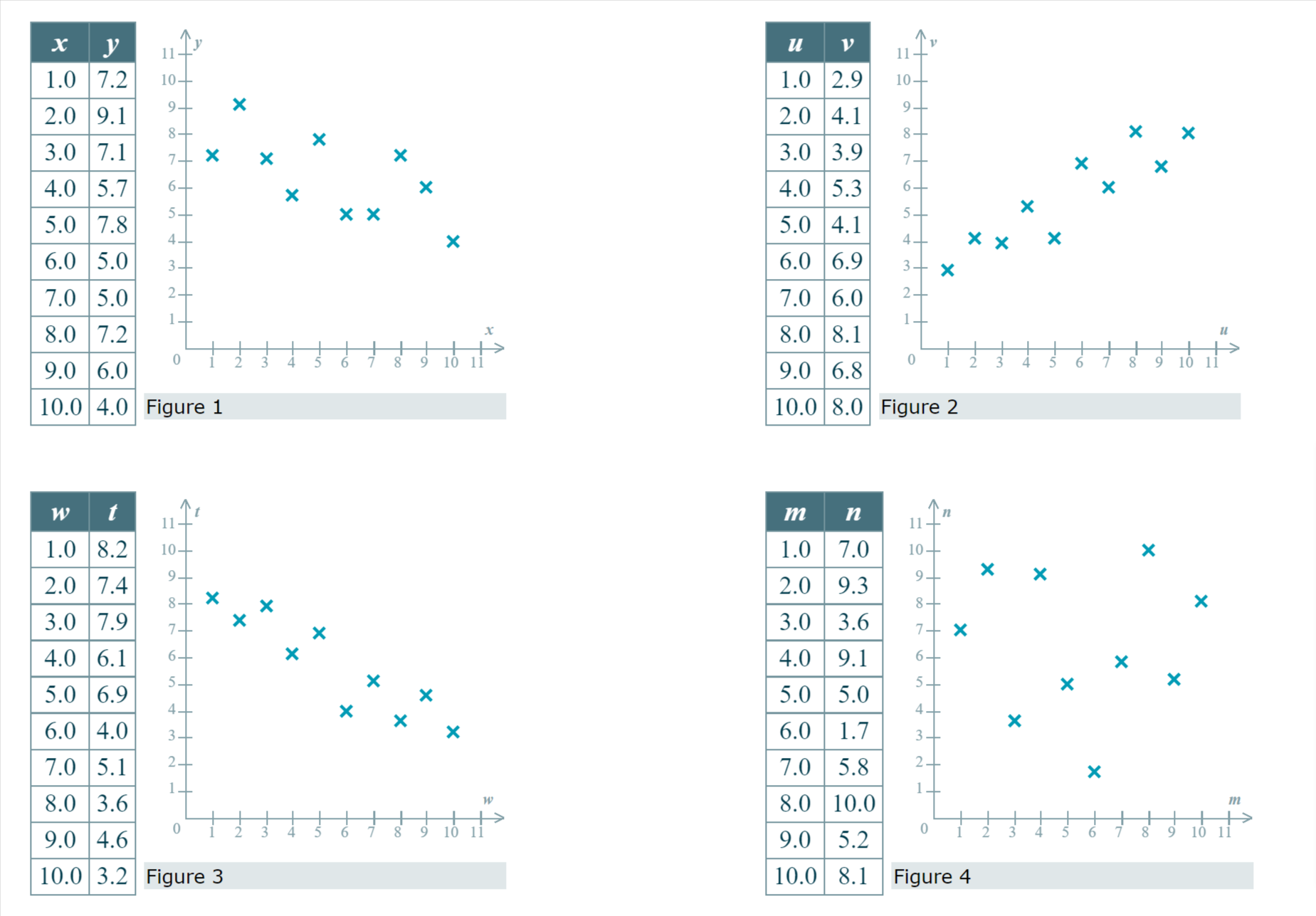
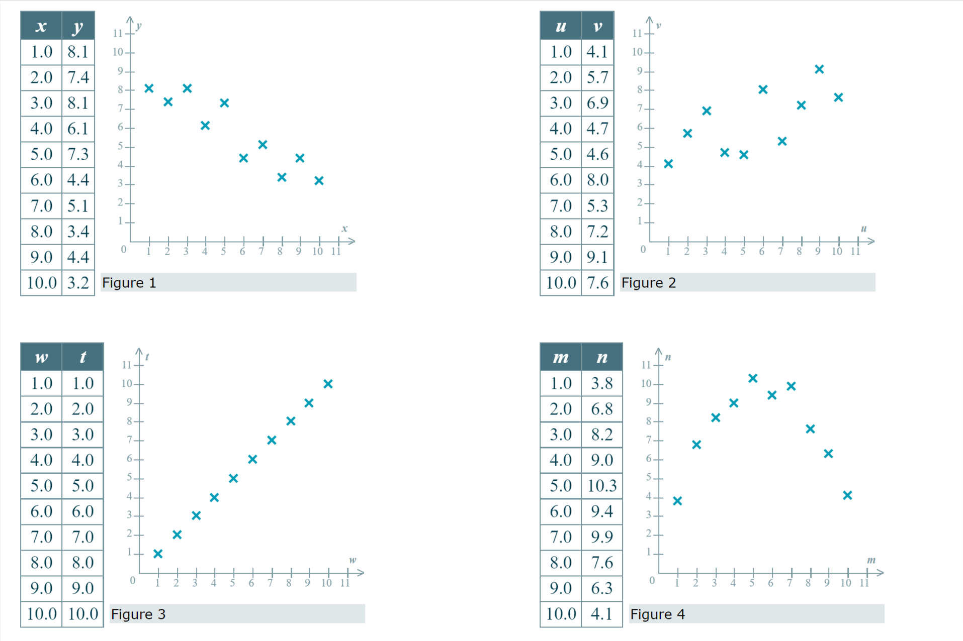
Below are four bivariate data sets and their scatter plots. (Note that all of the scatter plots are displayed with the same scale.) Each data set is made up of sample values drawn from a population.

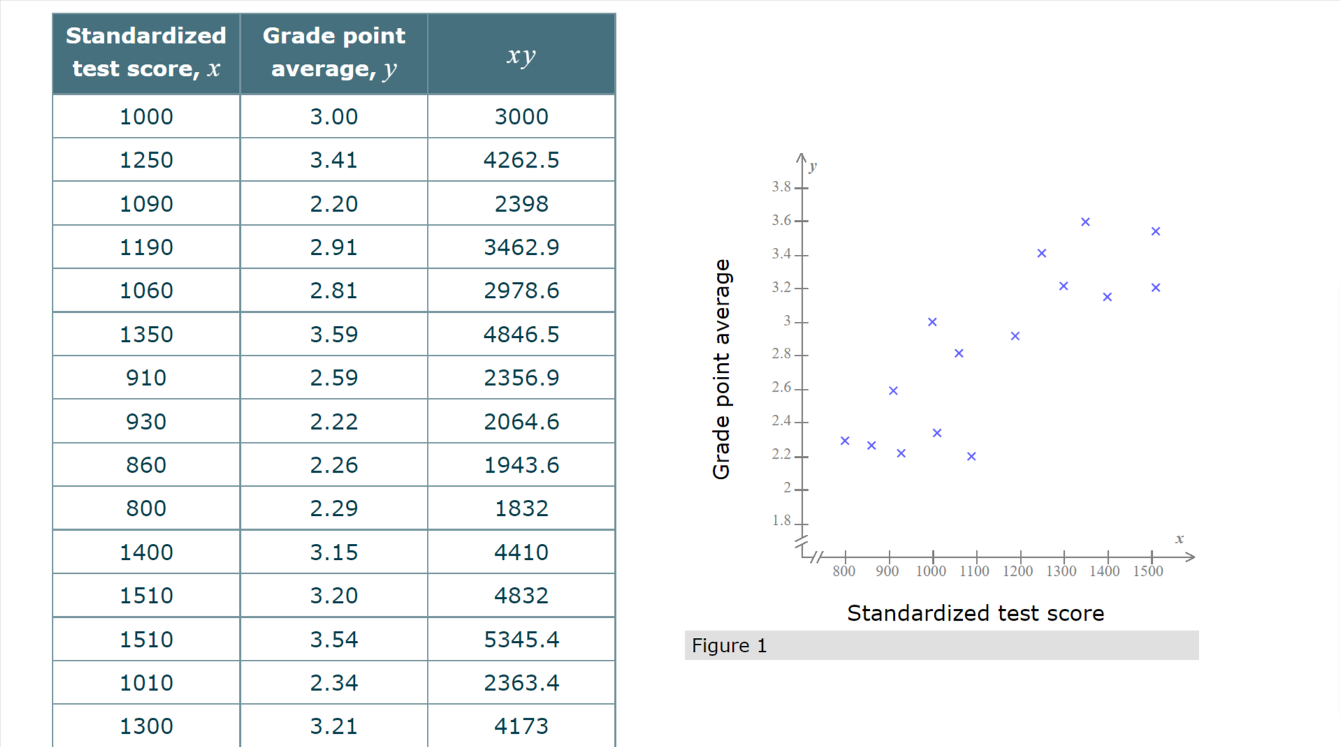
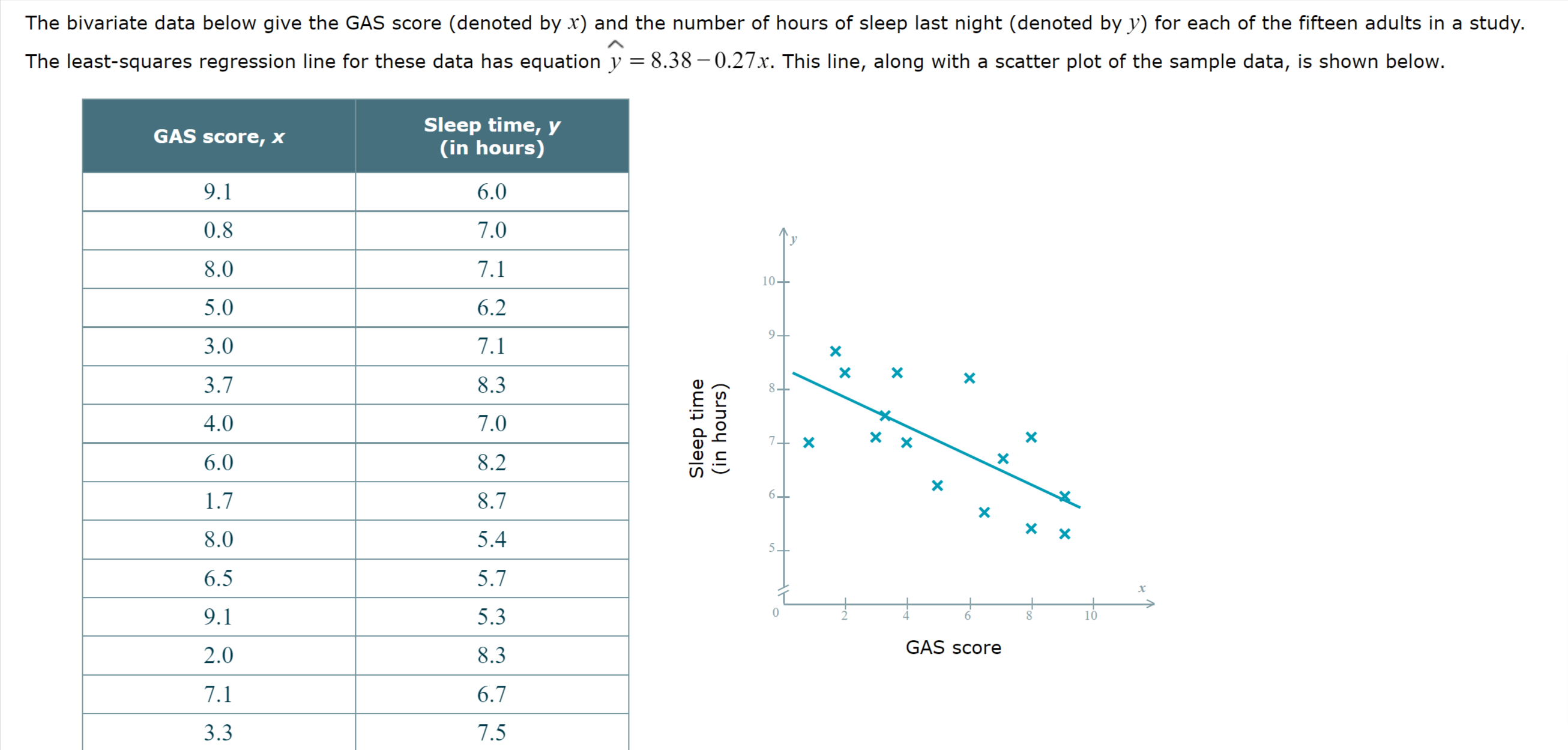
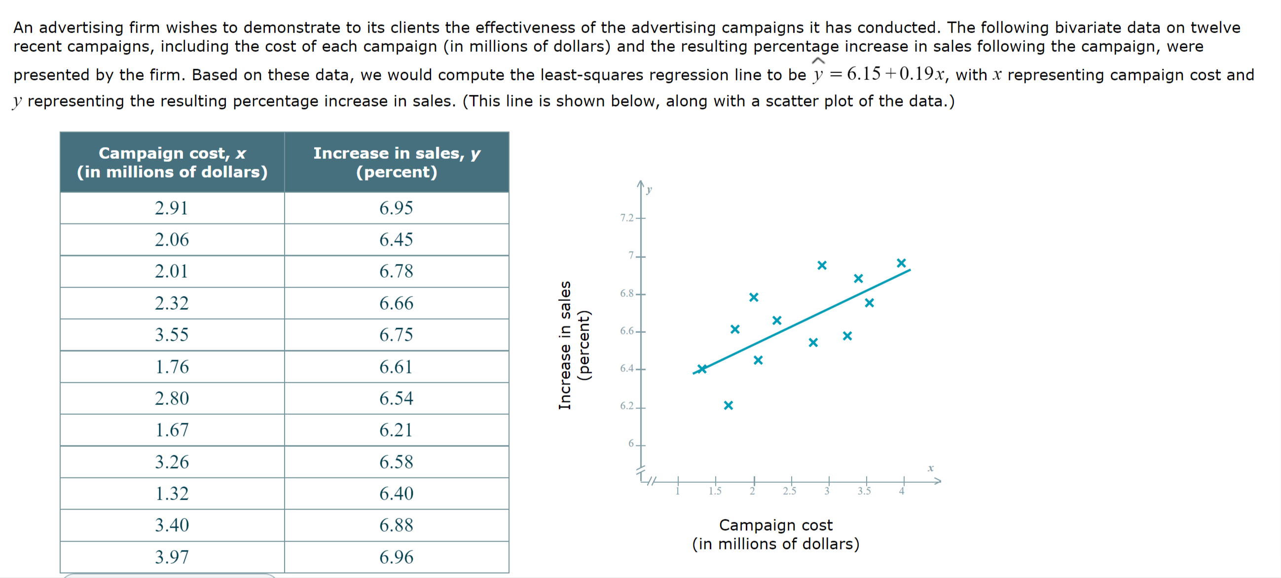
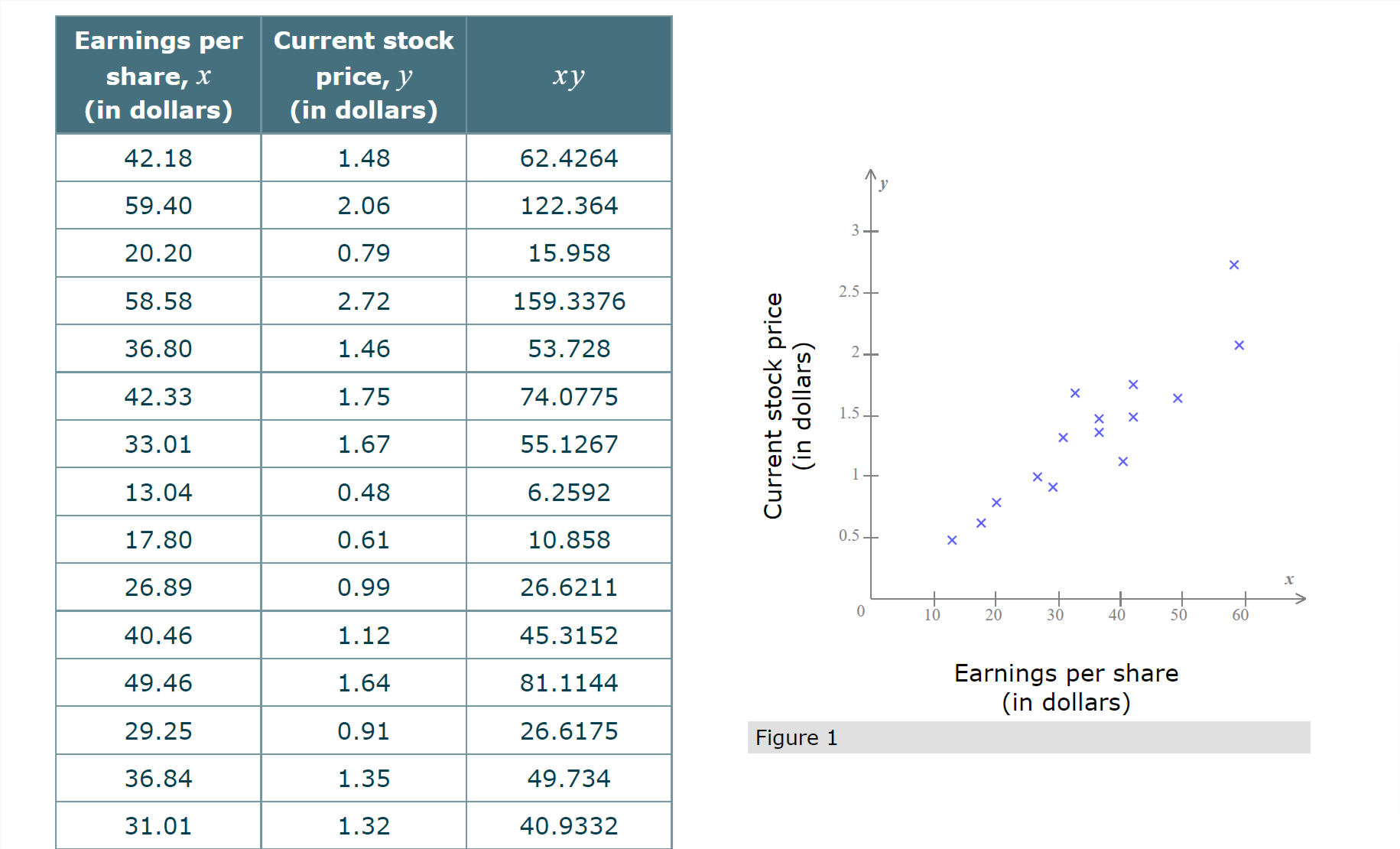
\fStandardized Grade point test score, I average, _1' A y 3.8... 3.6 x 3.4 x 3.2 X x 3 x 2.8 x 2.6 x 2.4... x 2.2 X x x Grade point average 2... 1.8... X // | | | | | l l I > 800 900 1000 1100 1200 1300 1400 1500 \\\\ Standardized test score Figure 1 1010 2.34 2363.4 1300 3.21 4173 The bivariate data below give the GAS score (denoted by x) and the number of hours of sleep last night (denoted by y) for each of the fifteen adults in a study. The least-squares regression line for these data has equation y = 8.38 -0.27x. This line, along with a scatter plot of the sample data, is shown below. GAS score, x Sleep time, y (in hours) 9.1 6.0 0.8 7.0 8.0 7.1 10- 5.0 6.2 9- 3.0 7.1 X X 3.7 8.3 X 4.0 7.0 (in hours) Sleep time 7- X X > X 6.0 8.2 X 1.7 8.7 6- X 8.0 5.4 X X 5- 6.5 5.7 9.1 5.3 8 2.0 8.3 GAS score 7.1 6.7 3.3 7.5An advertising firm wishes to demonstrate to its clients the effectiveness of the advertising campaigns it has conducted. The following bivariate data on twelve recent campaigns, including the cost of each campaign (in millions of dollars) and the resulting percentage increase in sales following the campaign, were A presented by the firm. Based on these data, we would compute the least-squares regression line to be y = 6.15 +0.19x, with x representing campaign cost and y representing the resulting percentage increase in sales. (This line is shown below, along with a scatter plot of the data.) Campaign cost, x Increase in sales, y (in millions of dollars) (percent) y 2.91 6.95 7.2 2.06 6.45 7 2.01 6.78 m 2.32 6.66 A 6'8 3.55 6.75 E 5 6-6 w 8 1.76 6.61 g g 6.4 2.80 6.54 g 62 x 1.67 6.21 5 3.26 6.58 X 1,, t l I i I . i 1.32 640 l 1.5 2 25 3 35 4 3.40 6.88 Campaign cost 3 97 6 96 (in millions of dollars) \fEarnings per Current stock share, .1" price, y (in dollars) (in dollars) 1.48 62.4264 A .V 59.40 2.06 122.364 3 20.20 0.79 15.958 x 2.72 159.3376 3 25 'E 1.46 53.728 Q1; 2- x x a. U m x 1.75 74.0775 .9 =0 x x u: .U 1.5 X x 1.67 55.1267 '5 c x " '1J C x t 1 x 0.48 6.2592 5 x x 0.61 10.858 0.5 x x 0 10 20 30 40 50 60 40.46 1.12 45.3152 49.46 1.64 81.1144 Earnings Per share (In dollars) 29.25 0.91 26.6175 Figure 1 1.35 49.734 40.9332