Q3 and Q4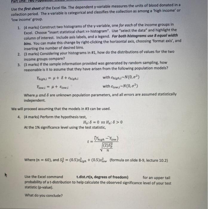

The data provided to answer the question starts here

page 1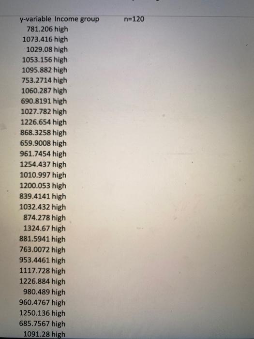

page 2

page 3

page 4

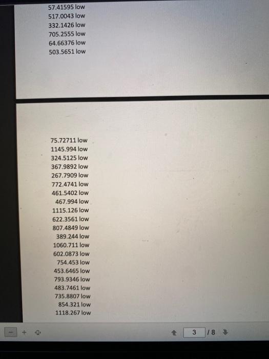
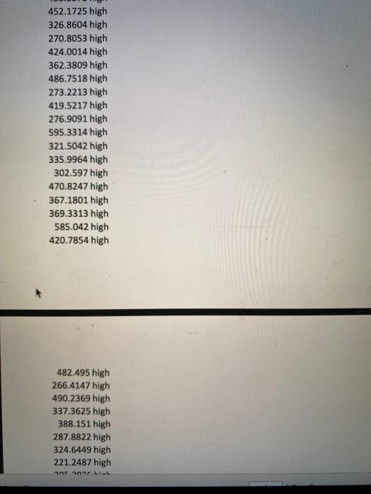
Use the first sheet of the Excel file. The dependent y-variable measures the units of blood donated in a collection period. The x-variable is categorical and classifies the collection as among a 'high income' or low income' group. 1. (4 marks) Construct two histograms of the y-variable, one for each of the income groups in Excel. Choose "insert statistical chart >> histogram". Use "select the data" and highlight the column of interest. Include axis labels, and a legend. For both histograms use 8 equal width bins. You can make this change by right-clicking the horizontal axis, choosing 'format axis', and inserting the number of desired bins. 2. (3 marks) Considering your histograms in #1, how do the distributions of values for the two income groups compare? 3. (3 marks) If the sample information provided was generated by random sampling, how reasonable is it to assume that they have arisen from the following population models? Ynight = x+ 8 + Enign with Enig~N(0,0%) Yiowi = 4+ Etow. with Erow :~N(0,0%) Where j and 8 are unknown population parameters, and all errors are assumed statistically independent. We will proceed assuming that the models in #3 can be used. 4. (4 marks) Perform the hypothesis test, H:8 = 0 vs H:8 > At the 1% significance level using the test statistic, Tyhigh - Yow) (2), 72 Where (n = 60), and S3 = (0.5)sign + (0.5)sow (formula on slide 8-9, lecture 10.2) Use the Excel command t.dist.rt(x, degrees of freedom) for an upper tail probability of a t-distribution to help calculate the observed significance level of your test statistic (p-value). What do you conclude? n=120 y-variable Income group 781.206 high 1073.416 high 1029.08 high 1053.156 high 1095.882 high 753.2714 high 1060.287 high 690.8191 high 1027.782 high 1226.654 high 868.3258 high 659.9008 high 961.7454 high 1254.437 high 1010.997 high 1200.053 high 839.4141 high 1032.432 high 874.278 high 1324.67 high 881.5941 high 763.0072 high 953.4461 high 1117.728 high 1226.884 high 980.489 high 960.4767 high 1250.136 high 685.7567 high 1091.28 high 452.1725 high 326.8604 high 270.8053 high 424.0014 high 362.3809 high 486.7518 high 273.2213 high 419.5217 high 276.9091 high 595.3314 high 321.5042 high 335.9964 high 302.597 high 470.8247 high 367.1801 high 369.3313 high 585.042 high 420.7854 high 482.495 high 266.4147 high 490.2369 high 337.3625 high 388.151 high 287.8822 high 324.6449 high 221.2487 high A DALIL 305.2936 high 344.7737 high 432.7558 high O low 210.1243 low 143.6194 low 179.7334 low 243.8226 low O low 282.4301 low O low 233.6726 low 531.9803 low O low Olow 134.618 low 573.6553 low 208.4955 low 492.0802 low O low 286.6473 low 49.41689 low 725.0049 low 60.39114 low O low 168.1692 low 414.5925 low 624.3264 low 254.7335 low 224.7151 low 659.2043 low O low 420.9199 low 615.6633 low 601.5175 low 225.5813 low CARE 57.41595 low 517.0043 low 332.1426 low 705.2555 low 64.66376 low 503.5651 low 75.72711 low 1145.994 low 324.5125 low 367.9892 low 267.7909 low 772.4741 low 461.5402 low 467.994 low 1115.126 low 622.3561 low 807.4849 low 389.244 low 1060.711 low 602.0873 low 754.453 low 453.6465 low 793.9346 low 483.7461 low 735.8807 low 854.321 low 1118.267 low 2 3 / 8 3 Use the first sheet of the Excel file. The dependent y-variable measures the units of blood donated in a collection period. The x-variable is categorical and classifies the collection as among a 'high income' or low income' group. 1. (4 marks) Construct two histograms of the y-variable, one for each of the income groups in Excel. Choose "insert statistical chart >> histogram". Use "select the data" and highlight the column of interest. Include axis labels, and a legend. For both histograms use 8 equal width bins. You can make this change by right-clicking the horizontal axis, choosing 'format axis', and inserting the number of desired bins. 2. (3 marks) Considering your histograms in #1, how do the distributions of values for the two income groups compare? 3. (3 marks) If the sample information provided was generated by random sampling, how reasonable is it to assume that they have arisen from the following population models? Ynight = x+ 8 + Enign with Enig~N(0,0%) Yiowi = 4+ Etow. with Erow :~N(0,0%) Where j and 8 are unknown population parameters, and all errors are assumed statistically independent. We will proceed assuming that the models in #3 can be used. 4. (4 marks) Perform the hypothesis test, H:8 = 0 vs H:8 > At the 1% significance level using the test statistic, Tyhigh - Yow) (2), 72 Where (n = 60), and S3 = (0.5)sign + (0.5)sow (formula on slide 8-9, lecture 10.2) Use the Excel command t.dist.rt(x, degrees of freedom) for an upper tail probability of a t-distribution to help calculate the observed significance level of your test statistic (p-value). What do you conclude? n=120 y-variable Income group 781.206 high 1073.416 high 1029.08 high 1053.156 high 1095.882 high 753.2714 high 1060.287 high 690.8191 high 1027.782 high 1226.654 high 868.3258 high 659.9008 high 961.7454 high 1254.437 high 1010.997 high 1200.053 high 839.4141 high 1032.432 high 874.278 high 1324.67 high 881.5941 high 763.0072 high 953.4461 high 1117.728 high 1226.884 high 980.489 high 960.4767 high 1250.136 high 685.7567 high 1091.28 high 452.1725 high 326.8604 high 270.8053 high 424.0014 high 362.3809 high 486.7518 high 273.2213 high 419.5217 high 276.9091 high 595.3314 high 321.5042 high 335.9964 high 302.597 high 470.8247 high 367.1801 high 369.3313 high 585.042 high 420.7854 high 482.495 high 266.4147 high 490.2369 high 337.3625 high 388.151 high 287.8822 high 324.6449 high 221.2487 high A DALIL 305.2936 high 344.7737 high 432.7558 high O low 210.1243 low 143.6194 low 179.7334 low 243.8226 low O low 282.4301 low O low 233.6726 low 531.9803 low O low Olow 134.618 low 573.6553 low 208.4955 low 492.0802 low O low 286.6473 low 49.41689 low 725.0049 low 60.39114 low O low 168.1692 low 414.5925 low 624.3264 low 254.7335 low 224.7151 low 659.2043 low O low 420.9199 low 615.6633 low 601.5175 low 225.5813 low CARE 57.41595 low 517.0043 low 332.1426 low 705.2555 low 64.66376 low 503.5651 low 75.72711 low 1145.994 low 324.5125 low 367.9892 low 267.7909 low 772.4741 low 461.5402 low 467.994 low 1115.126 low 622.3561 low 807.4849 low 389.244 low 1060.711 low 602.0873 low 754.453 low 453.6465 low 793.9346 low 483.7461 low 735.8807 low 854.321 low 1118.267 low 2 3 / 8 3