Question 1

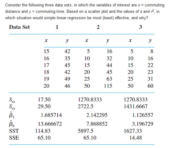
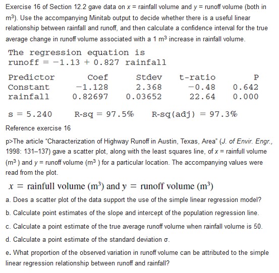
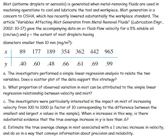
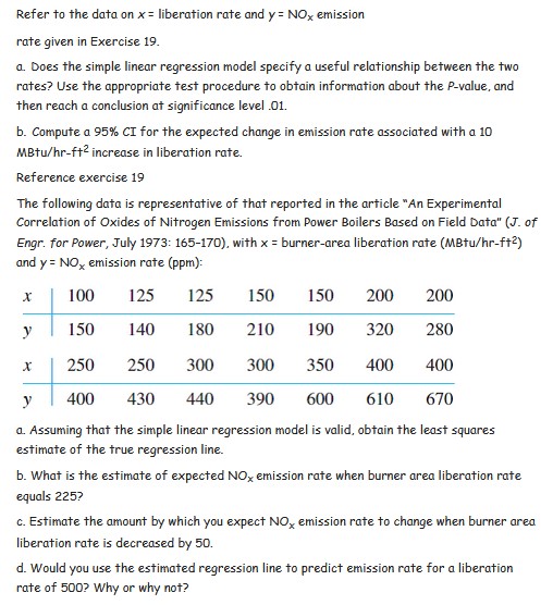
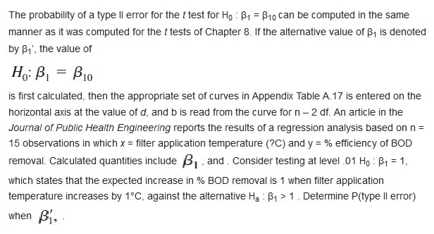
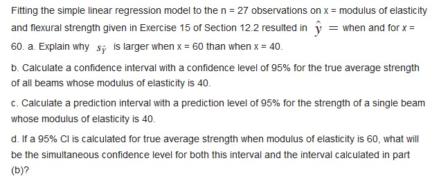
Consider the following three data sets, in which the variables of interest are r: commuting distance and v = commuting time. Based on a scatter plot and the values ofs and :3, in which situation would simple linear regression he most {least} effective, and why? Data Set 1 I 15 16 1'? 13 19 20 1150 29.50 1.6857 14 [3.6666312 114.33 65.10 42 35 45 42 49 2 I .F 5 16 10 32 15 44 2|]| 45 25 63 5|] 1 15 12203333 2122.5 2. 142295 "1.863852 53915 65. I 0 3 I .1' 5 3 10 16 15 22 20 23 25 3 l 50 60 125'03333 I43 1 .666? 1.12655? 3.196229 1627.33 14.43 Exercise 16 of Section 12.2 gave data on x = rainfall volume and y = runoff volume (both in m3). Use the accompanying Minitab output to decide whether there is a useful linear relationship between rainfall and runoff, and then calculate a confidence interval for the true average change in runoff volume associated with a 1 me increase in rainfall volume. The regression equation is runoff = -1.13 + 0. 827 rainfall Predictor Coef Stdev t-ratio P Constant -1 . 128 2.368 -0.48 0 . 642 rainfall 0. 82697 0. 03652 22 .64 0. 000 s = 5. 240 R-sq = 97.5% R-sq (adj ) = 97.3% Reference exercise 16 p>The article "Characterization of Highway Runoff in Austin, Texas, Area" (J. of Envir Engr., 1998: 131-137) gave a scatter plot, along with the least squares line, of x = rainfull volume (m3 ) and y = runoff volume (m3 ) for a particular location. The accompanying values were read from the plot. x = rainfull volume (m3) and y = runoff volume (m3) a. Does a scatter plot of the data support the use of the simple linear regression model? b. Calculate point estimates of the slope and intercept of the population regression line. c. Calculate a point estimate of the true average runoff volume when rainfall volume is 50. d. Calculate a point estimate of the standard deviation o. e. What proportion of the observed variation in runoff volume can be attributed to the simple linear regression relationship between runoff and rainfall?Mist (airborne droplets or aerosols) is generated when metal-removing fluids are used in machining operations to cool and lubricate the tool and workpiece. Mist generation is a concern to OSHA, which has recently lowered substantially the workplace standard. The article "Variables Affecting Mist Generaton from Metal Removal Fluids" (Lubrication Engr., 2002: 10-17) gave the accompanying data on x= fluid-flow velocity for a 5% soluble oil (cm/sec) and y = the extent of mist droplets having diameters smaller than 10 mm (mg/m3): 89 177 189 354 362 442 965 .40 .60 .48 .66 .61 .69 .99 a. The investigators performed a simple linear regression analysis to relate the two variables. Does a scatter plot of the data support this strategy? b. What proportion of observed variation in mist can be attributed to the simple linear regression relationship between velocity and mist? c. The investigators were particularly interested in the impact on mist of increasing velocity from 100 to 1000 (a factor of 10 corresponding to the difference between the smallest and largest x values in the sample). When x increases in this way, is there substantial evidence that the true average increase in y is less than .6? d. Estimate the true average change in mist associated with a 1 cm/sec increase in velocity, and do so in a way that conveys information about precision and reliability.Refer to the data on x = liberation rate and y = NO, emission rate given in Exercise 19. a. Does the simple linear regression model specify a useful relationship between the two rates? Use the appropriate test procedure to obtain information about the P-value, and then reach a conclusion at significance level .01. b. Compute a 95% CI for the expected change in emission rate associated with a 10 MBtu/hr-ftz increase in liberation rate. Reference exercise 19 The following data is representative of that reported in the article "An Experimental Correlation of Oxides of Nitrogen Emissions from Power Boilers Based on Field Data" (J. of Engr. for Power, July 1973: 165-170), with x = burner-area liberation rate (MBtu/hr-f+2) and y = NO, emission rate (ppm): X 100 125 125 150 150 200 200 y 150 140 180 210 190 320 280 X 250 250 300 300 350 400 400 y 400 430 440 390 600 610 670 a. Assuming that the simple linear regression model is valid, obtain the least squares estimate of the true regression line. b. What is the estimate of expected NO, emission rate when burner area liberation rate equals 225? c. Estimate the amount by which you expect NO, emission rate to change when burner area liberation rate is decreased by 50. d. Would you use the estimated regression line to predict emission rate for a liberation rate of 500? Why or why not?The probability of a type ll error for the t test for Ho : 1 = $10 can be computed in the same manner as it was computed for the t tests of Chapter 8. If the alternative value of B, is denoted by B1', the value of Ho: B1 = Bio is first calculated, then the appropriate set of curves in Appendix Table A.17 is entered on the horizontal axis at the value of d, and b is read from the curve for n - 2 df. An article in the Journal of Public Health Engineering reports the results of a regression analysis based on n = 15 observations in which x = filter application temperature (?C) and y = % efficiency of BOD removal. Calculated quantities include 3, and . Consider testing at level .01 Ho : B1 = 1, which states that the expected increase in % BOD removal is 1 when filter application temperature increases by 1'C, against the alternative Ha : B, > 1 . Determine P(type ll error) whenFitting the simple linear regression model to the n = 2? observations on x = modulus of elasticity and exural strength given in Exercise 15 of Section 12.2 resulted in it 2 when and for r: 613. a. Explain why 3;, is larger when x = Ed than when x = 4d. b. Calculate a confidence interval with a confidence level of 95% for the true average strength of all beams whose modulus of elasticity is 4G. c. Calculate a prediction interval with a prediction level of 95% for the strength of a single beam whose modulus of elasticity is 40. d. If a 95% Cl is calculated for true average strength when modulus of elasticity is t], what will be the simuttaneous condence level for both this interval and the interval calculated in part {D}