QUESTION 1

The attached data set provides information in Eviews format about the following variables

Gross Domestic Product =GDP Velocity of money = M2V Federal Debt as % of GDP =debt Gross private saving = save

Run the regression of GDP on M2V and Debt and answer the following questions.

homework all.wf1

QUESTION 2

Use the Eviews results in question one and choose the correct answer.

		the sign of M2V and debt coefficients make sense because as the velocity of money increases, the debt increases too.
		the sign of M2V and debt coefficients make sense because as the velocity of money increases so does GDP and as the debt increases, so does GDP increases.
		the sign of debt is not correct. it should be positive
		the sign of velocity is not correct, it should be negative.

QUESTION 3

Interpret the coefficient of M2V

		As GDP increase, M2V increase as much as 2761.53 .
		If Debt increases by, GDP will increase by 232.07 units.
		If M2V increases by I unit , GDP will increase by 2761 units, assuming Debt remains constant.
		If GDP increases by 1 units, Debt will increase by 232.07 units, assuming all other variables remain constant.

QUESTION 4

The R sqaured of the regression shows that:

		the regression is a good fit.
		If all the variables increase by 1 unit GDP will increase by 81%
		81% of variation in GDP around its mean is explained by M2V and Debt
		we should not use R squared to measure goodness of fit.

QUESTION 5

Choose one of the following answers:

		The null hypothesis for T test in front of M2v is H0: the sample slope = 0
		The null hypothesis for T test in front of M2v is H0: GDP has no effect on M2V in reality
		The null hypothesis for T test in front of debt is H0: Debt has no effect on GDP in reality.
		The null hypothesis for T test in front of debt is H0: Debt has a significant effect on GDP

QUESTION 6

the degree of freedom for the estimated t values is

		174
		172
		171
		170

QUESTION 7

The Estimated T values implies:

		We can reject the null hypothesis at 5% level of significance.
		We should Drop M2V and Debt from the regression.
		the effects of M2V and Debt on GDP are statistically different from zero at 5% level of significance.
		the effects of M2V and Debt on GDP are statistically zero at 5% level of significance.

QUESTION 8

choosing the significance level of 5% means

		5% of times we are wrong when we reject the null.
		5% of times we are correct when we reject the null.
		5% of times we are correct when we can not reject the null.
		5% of times we are wrong when we can not reject the null.

QUESTION 10

Choose one of the following answers.

		The estimated F statistic of the regression tests the null hypothesis that R squaredof the regression is significantly different from zero.
		The estimated F statistic of the regression tests the null hypothesis that the joint effect of all the variables in the regression is significantly different from zero.
		The F test is one sided test.
		All other answers are correct.

QUESTION 11

choose one of the following answers.

		The degree of freedom of the estimated F in the regression is 3, 174 and it rejects the null hypothesis that R squared is zero.
		The degree of freedom of the estimated F in the regression is 2, 171 and it rejects the null hypothesis that R squared is zero.
		The degree of freedom of the estimated F in the regression is 3, 172 and it rejects the null hypothesis that R squared is zero.
		The degree of freedom of the estimated F in the regression is 2, 171 and it can not reject the null hypothesis that R squared is zero.

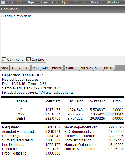
a File Edit Object View Proc Quick Options Add-ins WindowH Command LS gdp c m2v debt CommandCapture View Proc Object Print Name Freeze Estimate Forecast Stats Resids Dependent Variable: GDP Method: Least Squares Date: 10/04/18 Time: 12:56 Sample (adjusted): 1970Q1 201302 Included observations: 174 after adjustments Variable Coefficient Std. Error t-Statistic Prob M2V DEBT 10171.75 1824.649 -5.574637 0.0000 2761.537 963.5775 2.865921 0.0047 232.0750 8.704252 26.66225 0.0000 R-squared Adjusted R-squared S.E. of regression Sum squared resid Log likelihood F-statistic Prob(F-statistic) 0.813159 Mean dependent var 0.810974 S.D. dependent var 2084.943 Akaike info criterion 7.43E+08 Schwarz criterion 1575.177 Hannan-Quinn criter 372.1079 Durbin-Watson stat 0.000000 7270.325 4795.490 18.13996 18.19443 18.16206 0.016902