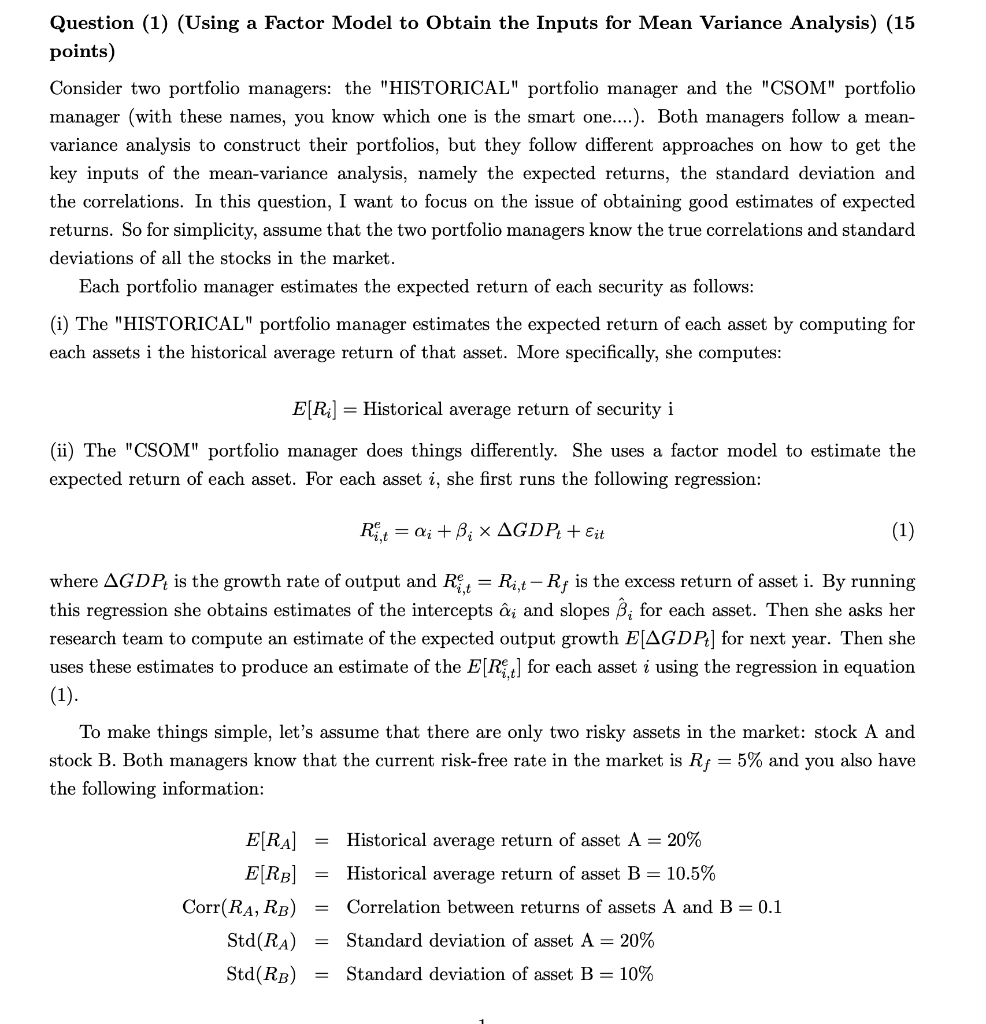
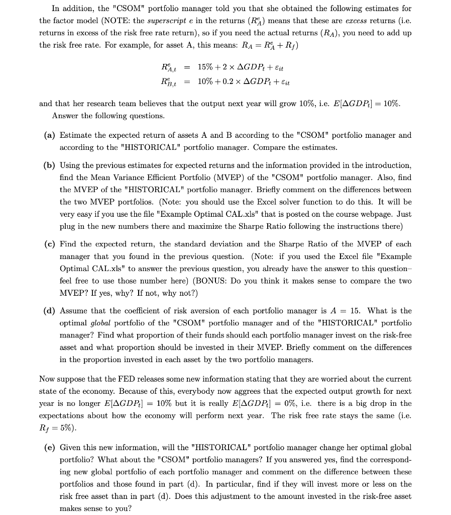
Question (1) (Using a Factor Model to obtain the Inputs for Mean Variance Analysis) (15 points) Consider two portfolio managers: the "HISTORICAL" portfolio manager and the "CSOM" portfolio manager (with these names, you know which one is the smart one...). Both managers follow a mean- variance analysis to construct their portfolios, but they follow different approaches on how to get the key inputs of the mean-variance analysis, namely the expected returns, the standard deviation and the correlations. In this question, I want to focus on the issue of obtaining good estimates of expected returns. So for simplicity, assume that the two portfolio managers know the true correlations and standard deviations of all the stocks in the market. Each portfolio manager estimates the expected return of each security as follows: (i) The "HISTORICAL" portfolio manager estimates the expected return of each asset by computing for each assets i the historical average return of that asset. More specifically, she computes: E[Ri] = Historical average return of security i (ii) The "CSOM" portfolio manager does things differently. She uses a factor model to estimate the expected return of each asset. For each asset i, she first runs the following regression: Ri,t = di +B; x AGDP+ + Eit (1) where AGDP is the growth rate of output and R, = Rint-Rf is the excess return of asset i. By running this regression she obtains estimates of the intercepts i and slopes B; for each asset. Then she asks her research team to compute an estimate of the expected output growth E[AGDP] for next year. Then she uses these estimates to produce an estimate of the E[RE,] for each asset i using the regression in equation (1). To make things simple, let's assume that there are only two risky assets in the market: stock A and stock B. Both managers know that the current risk-free rate in the market is Rs = 5% and you also have the following information: = E[RA] E[RB] Corr(RA, RB) Std(RA) Std(RB) Historical average return of asset A = 20% Historical average return of asset B = 10.5% Correlation between returns of assets A and B = 0.1 = = Standard deviation of asset A= 20% Standard deviation of asset B= 10% In addition, the "CSOM" portfolio manager told you that she obtained the following estimates for the factor model (NOTE: the superscript e in the returns (RA) means that these are excess returns (i.e. returns in excess of the risk free rate return), so if you need the actual returns (RA), you need to add up the risk free rate. For example, for asset A, this means: RA= RA + R) RAL RB 15% + 2 X AGDP + Eit 10% +0.2 X AGDP + Eit and that her research team believes that the output next year will grow 10%, i.e. E(AGDPt] = 10%. Answer the following questions. (a) Estimate the expected return of assets A and B according to the "CSOM" portfolio manager and according to the "HISTORICAL" portfolio manager. Compare the estimates. (b) Using the previous estimates for expected returns and the information provided in the introduction, find the Mean Variance Efficient Portfolio (MVEP) of the "CSOM" portfolio manager. Also, find the MVEP of the "HISTORICAL" portfolio manager. Briefly comment on the differences between the two MVEP portfolios. (Note: you should use the Excel solver function to do this. It will be very easy if you use the file "Example Optimal CAL.xls" that is posted on the course webpage. Just plug in the new numbers there and maximize the Sharpe Ratio following the instructions there) (c) Find the expected return, the standard deviation and the Sharpe Ratio of the MVEP of each manager that you found in the previous question. (Note: if you used the Excel file "Example Optimal CAL.xls" to answer the previous question, you already have the answer to this question- feel free to use those number here) (BONUS: Do you think it makes sense to compare the two MVEP? If yes, why? If not, why not?) (d) Assume that the coefficient of risk aversion of each portfolio manager is A = 15. What is the optimal global portfolio of the "CSOM" portfolio manager and of the "HISTORICAL" portfolio manager? Find what proportion of their funds should each portfolio manager invest on the risk-free asset and what proportion should be invested in their MVEP. Briefly comment on the differences in the proportion invested in each asset by the two portfolio managers. Now suppose that the FED releases some new information stating that they are worried about the current state of the economy. Because of this, everybody now aggrees that the expected output growth for next year is no longer EJAGDP] = 10% but it is really E[AGDP2] = 0%, i.e. there is a big drop in the expectations about how the economy will perform next year. The risk free rate stays the same (i.e. Rg = 5%). (e) Given this new information, will the "HISTORICAL" portfolio manager change her optimal global portfolio? What about the "CSOM" portfolio managers? If you answered yes, find the correspond- ing new global portfolio of each portfolio manager and comment on the difference between these portfolios and those found in part (d). In particular, find if they will invest more or less on the risk free asset than in part (d). Does this adjustment to the amount invested in the risk-free asset makes sense to you? Question (1) (Using a Factor Model to obtain the Inputs for Mean Variance Analysis) (15 points) Consider two portfolio managers: the "HISTORICAL" portfolio manager and the "CSOM" portfolio manager (with these names, you know which one is the smart one...). Both managers follow a mean- variance analysis to construct their portfolios, but they follow different approaches on how to get the key inputs of the mean-variance analysis, namely the expected returns, the standard deviation and the correlations. In this question, I want to focus on the issue of obtaining good estimates of expected returns. So for simplicity, assume that the two portfolio managers know the true correlations and standard deviations of all the stocks in the market. Each portfolio manager estimates the expected return of each security as follows: (i) The "HISTORICAL" portfolio manager estimates the expected return of each asset by computing for each assets i the historical average return of that asset. More specifically, she computes: E[Ri] = Historical average return of security i (ii) The "CSOM" portfolio manager does things differently. She uses a factor model to estimate the expected return of each asset. For each asset i, she first runs the following regression: Ri,t = di +B; x AGDP+ + Eit (1) where AGDP is the growth rate of output and R, = Rint-Rf is the excess return of asset i. By running this regression she obtains estimates of the intercepts i and slopes B; for each asset. Then she asks her research team to compute an estimate of the expected output growth E[AGDP] for next year. Then she uses these estimates to produce an estimate of the E[RE,] for each asset i using the regression in equation (1). To make things simple, let's assume that there are only two risky assets in the market: stock A and stock B. Both managers know that the current risk-free rate in the market is Rs = 5% and you also have the following information: = E[RA] E[RB] Corr(RA, RB) Std(RA) Std(RB) Historical average return of asset A = 20% Historical average return of asset B = 10.5% Correlation between returns of assets A and B = 0.1 = = Standard deviation of asset A= 20% Standard deviation of asset B= 10% In addition, the "CSOM" portfolio manager told you that she obtained the following estimates for the factor model (NOTE: the superscript e in the returns (RA) means that these are excess returns (i.e. returns in excess of the risk free rate return), so if you need the actual returns (RA), you need to add up the risk free rate. For example, for asset A, this means: RA= RA + R) RAL RB 15% + 2 X AGDP + Eit 10% +0.2 X AGDP + Eit and that her research team believes that the output next year will grow 10%, i.e. E(AGDPt] = 10%. Answer the following questions. (a) Estimate the expected return of assets A and B according to the "CSOM" portfolio manager and according to the "HISTORICAL" portfolio manager. Compare the estimates. (b) Using the previous estimates for expected returns and the information provided in the introduction, find the Mean Variance Efficient Portfolio (MVEP) of the "CSOM" portfolio manager. Also, find the MVEP of the "HISTORICAL" portfolio manager. Briefly comment on the differences between the two MVEP portfolios. (Note: you should use the Excel solver function to do this. It will be very easy if you use the file "Example Optimal CAL.xls" that is posted on the course webpage. Just plug in the new numbers there and maximize the Sharpe Ratio following the instructions there) (c) Find the expected return, the standard deviation and the Sharpe Ratio of the MVEP of each manager that you found in the previous question. (Note: if you used the Excel file "Example Optimal CAL.xls" to answer the previous question, you already have the answer to this question- feel free to use those number here) (BONUS: Do you think it makes sense to compare the two MVEP? If yes, why? If not, why not?) (d) Assume that the coefficient of risk aversion of each portfolio manager is A = 15. What is the optimal global portfolio of the "CSOM" portfolio manager and of the "HISTORICAL" portfolio manager? Find what proportion of their funds should each portfolio manager invest on the risk-free asset and what proportion should be invested in their MVEP. Briefly comment on the differences in the proportion invested in each asset by the two portfolio managers. Now suppose that the FED releases some new information stating that they are worried about the current state of the economy. Because of this, everybody now aggrees that the expected output growth for next year is no longer EJAGDP] = 10% but it is really E[AGDP2] = 0%, i.e. there is a big drop in the expectations about how the economy will perform next year. The risk free rate stays the same (i.e. Rg = 5%). (e) Given this new information, will the "HISTORICAL" portfolio manager change her optimal global portfolio? What about the "CSOM" portfolio managers? If you answered yes, find the correspond- ing new global portfolio of each portfolio manager and comment on the difference between these portfolios and those found in part (d). In particular, find if they will invest more or less on the risk free asset than in part (d). Does this adjustment to the amount invested in the risk-free asset makes sense to you