Question 1 -

Using information in the question 5 from below please answer - researchers typically specify the alternative hypothesis to align with the expected outcome from the test, so rejection of the null hypothesis provides support for this outcome. Accordingly, would you specify the alternative hypothesis for the "neglected company effect" as positive or negative? Would you specify the alternative hypothesis for the "small company effect" as positive or negative? Based on the individual t-statistics for these coefficients, does it appear that either effect is supported by the evidence in these fitted models?

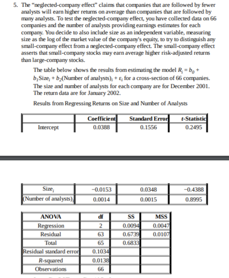
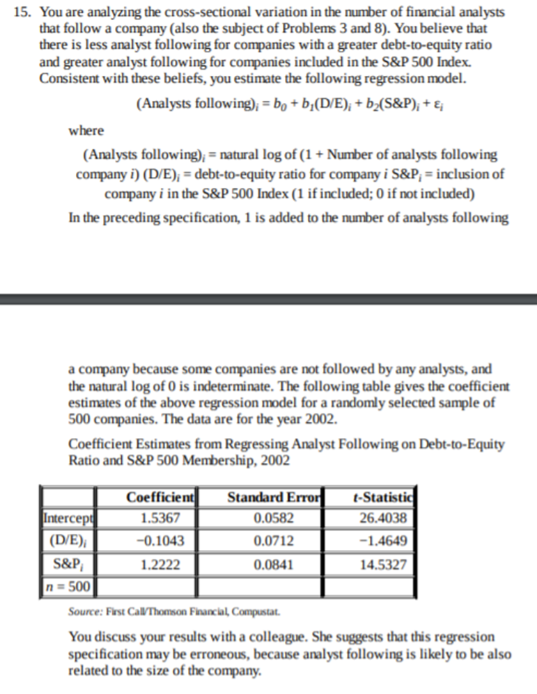
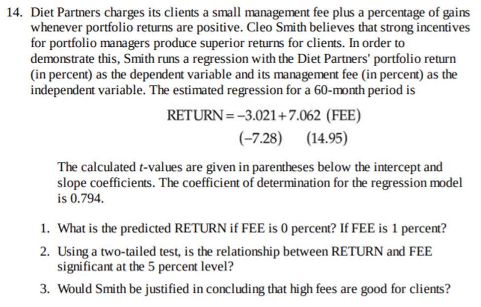
5. The "neglected-company effect" claims that companies that are followed by fewer analysts will earn higher returns on average than companies that are followed by many analysts. To test the neglected-company effect, you have collected data on 66 companies and the number of analysts providing earnings estimates for each company. You decide to also include size as an independent variable, measuring size as the log of the market value of the company's equity, to try to distinguish any small-company effect from a neglected-company effect. The small-company effect asserts that small-company stocks may earn average higher risk-adjusted returns than large-company stocks. The table below shows the results from estimating the model R; = bo + b, Size, + b2(Number of analysts); + , for a cross-section of 66 companies. The size and number of analysts for each company are for December 2001. The return data are for January 2002. Results from Regressing Returns on Size and Number of Analysts Coefficient Standard Error t-Statistic Intercept 0.0388 0.1556 0.2495 Size, -0.0153 0.0348 -0.4388 (Number of analysts) 0.0014 0.0015 0.8995 ANOVA df SS MSS Regression 2 0.0094 0.0047 Residual 63 0.6739 0.0107 Total 65 0.6833 Residual standard error 0.1034 R-squared 0.0138 Observations 6615. You are analyzing the cross-sectional variation in the number of financial analysts that follow a company (also the subject of Problems 3 and 8). You believe that there is less analyst following for companies with a greater debt-to-equity ratio and greater analyst following for companies included in the S&P 500 Index. Consistent with these beliefs, you estimate the following regression model. (Analysts following); = bo + b,(D/E); + b2(S&P); + &; where (Analysts following); = natural log of (1 + Number of analysts following company i) (D/E); = debt-to-equity ratio for company i S&P, = inclusion of company i in the S&P 500 Index (1 if included; 0 if not included) In the preceding specification, 1 is added to the number of analysts following a company because some companies are not followed by any analysts, and the natural log of 0 is indeterminate. The following table gives the coefficient estimates of the above regression model for a randomly selected sample of 500 companies. The data are for the year 2002. Coefficient Estimates from Regressing Analyst Following on Debt-to-Equity Ratio and S&P 500 Membership, 2002 Coefficient Standard Error t-Statistic Intercept 1.5367 0.0582 26.4038 (D/E); -0.1043 0.0712 -1.4649 S&P 1.2222 0.0841 14.5327 n = 500 Source: First Call/Thomson Financial, Compustat. You discuss your results with a colleague. She suggests that this regression specification may be erroneous, because analyst following is likely to be also related to the size of the company.14. Diet Partners charges its clients a small management fee plus a percentage of gains whenever portfolio returns are positive. Cleo Smith believes that strong incentives for portfolio managers produce superior returns for clients. In order to demonstrate this, Smith runs a regression with the Diet Partners' portfolio return (in percent) as the dependent variable and its management fee (in percent) as the independent variable. The estimated regression for a 60-month period is RETURN = -3.021+7.062 (FEE) (-7.28) (14.95) The calculated t-values are given in parentheses below the intercept and slope coefficients. The coefficient of determination for the regression model is 0.794. 1. What is the predicted RETURN if FEE is 0 percent? If FEE is 1 percent? 2. Using a two-tailed test, is the relationship between RETURN and FEE significant at the 5 percent level? 3. Would Smith be justified in concluding that high fees are good for clients