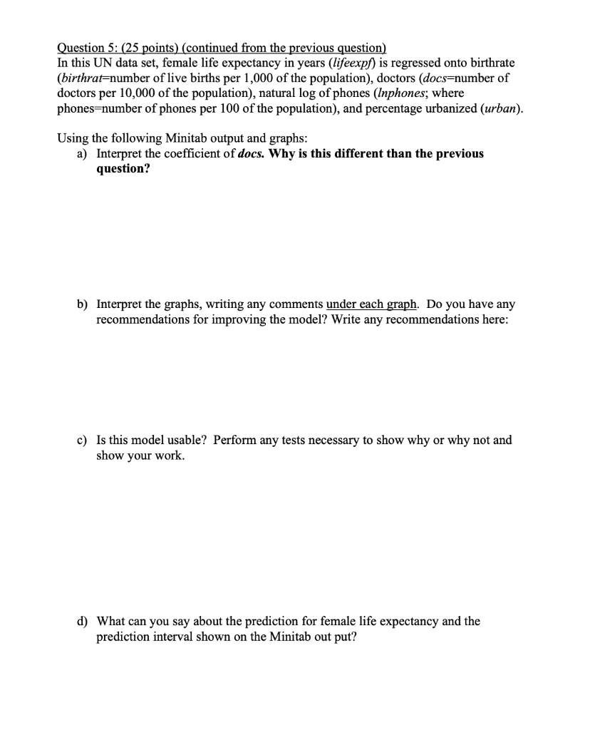
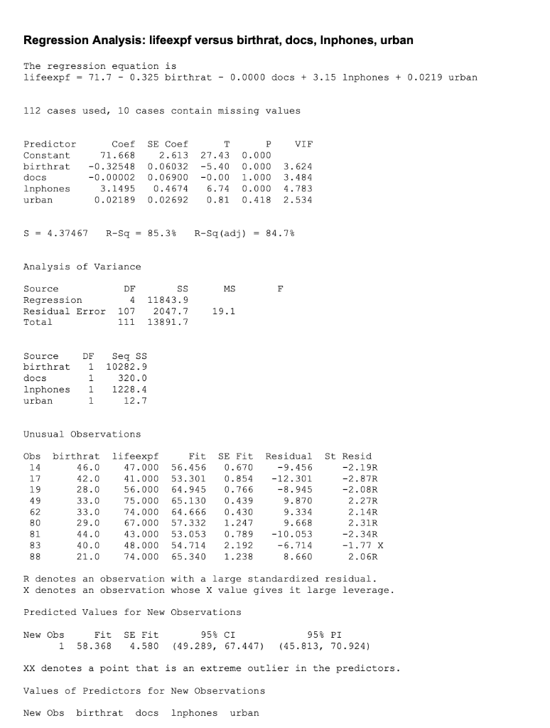
Question: Question 5: (25 points) (continued from the previous question) In this UN data set, female life expectancy in years (lifeexpf) is regressed onto birthrate (birthrat=number

Question 5: (25 points) (continued from theQuestion 5: (25 points) (continued from theQuestion 5: (25 points) (continued from theQuestion 5: (25 points) (continued from the

Question 5: (25 points) (continued from the previous question) In this UN data set, female life expectancy in years (lifeexpf) is regressed onto birthrate (birthrat=number of live births per 1,000 of the population), doctors (docs=number of doctors per 10,000 of the population), natural log of phones (Inphones; where phones=number of phones per 100 of the population), and percentage urbanized (urban). Using the following Minitab output and graphs: a) Interpret the coefficient of docs. Why is this different than the previous question? b) Interpret the graphs, writing any comments under each graph. Do you have any recommendations for improving the model? Write any recommendations here: c) Is this model usable? Perform any tests necessary to show why or why not and show your work d) What can you say about the prediction for female life expectancy and the prediction interval shown on the Minitab out put? Regression Analysis: lifeexpf versus birthrat, docs, Inphones, urban The regression equation is lifeexpf = 71.7 - 0.325 birthrat - 0.0000 docs + 3.15 Inphones + 0.0219 urban 112 cases used, 10 cases contain missing values VIF Predictor Constant birthrat docs lnphones urban Coef 71.668 -0.32548 -0.00002 3.1495 0.02189 SE Coef 2.613 0.06032 0.06900 0.4674 0.02692 T 27.43 -5.40 -0.00 6.74 0.81 P 0.000 0.000 1.000 0.000 0.418 3.624 3.484 4.783 2.534 S = 4.37467 R-Sq - 85.3% R-Sq(adj) = 84.78 Analysis of Variance MS F Source Regression Residual Error Total DF 4 107 111 SS 11843.9 2047.7 13891.7 19.1 Source birthrat docs Inphones urban DF 1 1 1 1 Seg ss 10282.9 320.0 1228.4 12.7 Unusual Observations Obs 14 17 19 49 62 80 81 83 88 birthrat lifeexpf Fit 46.0 47.000 56.456 42.0 41.000 53.301 28.0 56.000 64.945 33.0 75.000 65.130 33.0 74.000 64.666 29.0 67.000 57.332 44.0 43.000 53.053 40.0 48.000 54.714 21.0 74.000 65.340 SE Fit 0.670 0.854 0.766 0.439 0.430 1.247 0.789 2.192 1.238 Residual -9.456 -12.301 -8.945 9.870 9.334 9.668 -10.053 -6.714 8.660 St Resid -2.19R -2.87R -2.08R 2.27R 2.14R 2.31R -2.34R -1.77 X 2.06R R denotes an observation with a large standardized residual. X denotes an observation whose X value gives it large leverage. Predicted Values for New Observations New Obs 1 Fit 58.368 SE Fit 4.580 95% CI (49.289, 67.447) 95% PI (45.813, 70.924) xx denotes a point that is an extreme outlier in the predictors. Values of Predictors for New Observations New Obs birthrat docs Inphones urban 1 75.0 50.0 3.00 76.0 Scatterplot of lifeexpf vs birthrat, docs, Inphones, urban birthrat docs 80 - 70 60 - 50 40 lifeexpf 20 60 0 10 30 40 40 Inphones 20 urban 80 70 60 50 40 -2 0 2 4 0 25 50 75 100 Normal Probability Plot of the Residuals (response is life expr) 99.9 Histogram of the Residuals (response is lifeet) 30 25- 95 90 NO 70 60 50 40 20 15- 20 10 5 10 5 1 01 0 -10 -5 10 15 -10 -5 5 10 15 0 Residual Residual Residuals Versus the Fitted Values (response is life expf) 10 5 - 0 -5 -10- -15 50 55 60 65 70 Fitted Value 75 80 85

Step by Step Solution

There are 3 Steps involved in it

1 Expert Approved Answer
Step: 1 Unlock blur-text-image
Question Has Been Solved by an Expert!

Get step-by-step solutions from verified subject matter experts

Step: 2 Unlock
Step: 3 Unlock

Students Have Also Explored These Related General Management Questions!