QUESTION: EXAMPLE 5.3 IS ATTACHED

Everyone's heard about the five Great Lakes described in this lecture. However, not everyone knows that there is a sixth lake in the system, Lake St. Clair, that is located on the river connecting Lakes Huron and Erie. By the standards of most other lakes, it's more than adequate (V = 6.6 km3, A, = 1114 km2,H = 5.9 m, Q = 1 70.5 km3 yr I ). However, in the context of the Great Lakes, it's at best a "Very Good Lake." (a) Determine the responses of Lakes Huron, St. Clair, and Erie to an impulse flux of strontium (as described in Example 5.3) to Lake Huron. That is, compute the response as if the fallout fell only on Huron. (b) Use the dimensionless analysis described at the end of the lecture to justify omitting Lake St. Clair from the Great Lakes.

Compare the analytical solution with a numerical solution obtained using ode45. Include your code and a plot to show a comparison between analytical and numerical solutions.

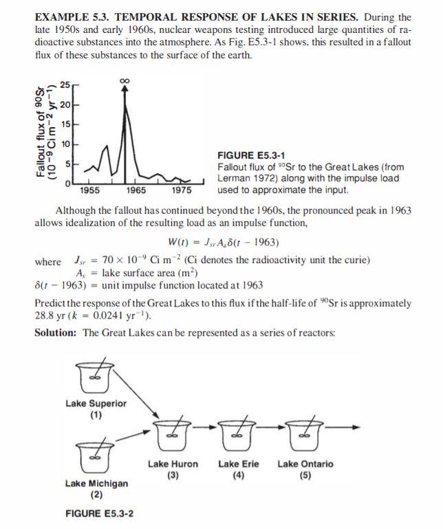
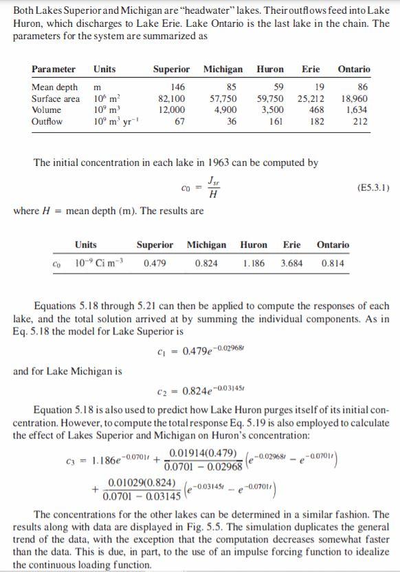
EXAMPLE 5.3. TEMPORAL RESPONSE OF LAKES IN SERIES. During the late 1950s and early 1960s, nuclear weapons testing introduced large quantities of ra- dioactive substances into the atmosphere. As Fig. E5.3-1 shows, this resulted in a fallout flux of these substances to the surface of the earth. 20 15 Fallout flux of 90 Sr (10 -9 Cim-2 yr -1) 10 W FIGURE E5.3-1 Fallout flux of Sr to the Great Lakes (from Lerman 1972) along with the impulse load 1955 1965 1975 used to approximate the input. Although the fallout has continued beyond the 1960s, the pronounced peak in 1963 allows idealization of the resulting load as an impulse function, W(t) = JsA8(1 - 1963) where J = 70 x 10-Gm? Ci denotes the radioactivity unit the curie) A, = lake surface area (m) 8(1 - 1963) = unit impulse function located at 1963 Predict the response of the Great Lakes to this flux if the half-life of Sr is approximately 28.8 yr (k = 0.0241 yr). Solution: The Great Lakes can be represented as a series of reactors: Lake Superior (1) Lake Huron (3) Lake Erie Lake Ontario (5) Lake Michigan (2) FIGURE E5.3-2 Both Lakes Superior and Michigan are "headwater" lakes. Their outflows feed into Lake Huron, which discharges to Lake Erie. Lake Ontario is the last lake in the chain. The parameters for the system are summarized as Parameter Units Mean depth m Surface area 10^m Volume 10m Outflow 10 myr Superior Michigan Huron Erie 146 85 59 19 82,100 57,750 59,750 25,212 12,000 3,500 468 67 36 Ontario 86 18,960 1.634 212 4.900 161 182 The initial concentration in each lake in 1963 can be computed by CO (E5.3.1) H where H = mean depth (m). The results are Units Co 109 Cim Superior Michigan Huron Erie Ontario 0.479 0.824 1.186 3.684 0.814 Equations 5.18 through 5.21 can then be applied to compute the responses of each lake, and the total solution arrived at by summing the individual components. As in Eq. 5.18 the model for Lake Superior is 9 = 0.479e-0.02968 and for Lake Michigan is C2 = 0.824e-0031451 1-2-007011) Equation 5.18 is also used to predict how Lake Huron purges itself of its initial con- centration. However, to compute the total response Eq. 5.19 is also employed to calculate the effect of Lakes Superior and Michigan on Huron's concentration: 0.01914(0.479) C3 = 1.186e-007011 -0.029684 0.0701 -0.02968 0.01029(0.824) le-0.03145 -0.07011 0.0701 - 0.03145 ) The concentrations for the other lakes can be determined in a similar fashion. The results along with data are displayed in Fig. 5.5. The simulation duplicates the general trend of the data, with the exception that the computation decreases somewhat faster than the data. This is due, in part, to the use of an impulse forcing function to idealize the continuous loading function. EXAMPLE 5.3. TEMPORAL RESPONSE OF LAKES IN SERIES. During the late 1950s and early 1960s, nuclear weapons testing introduced large quantities of ra- dioactive substances into the atmosphere. As Fig. E5.3-1 shows, this resulted in a fallout flux of these substances to the surface of the earth. 20 15 Fallout flux of 90 Sr (10 -9 Cim-2 yr -1) 10 W FIGURE E5.3-1 Fallout flux of Sr to the Great Lakes (from Lerman 1972) along with the impulse load 1955 1965 1975 used to approximate the input. Although the fallout has continued beyond the 1960s, the pronounced peak in 1963 allows idealization of the resulting load as an impulse function, W(t) = JsA8(1 - 1963) where J = 70 x 10-Gm? Ci denotes the radioactivity unit the curie) A, = lake surface area (m) 8(1 - 1963) = unit impulse function located at 1963 Predict the response of the Great Lakes to this flux if the half-life of Sr is approximately 28.8 yr (k = 0.0241 yr). Solution: The Great Lakes can be represented as a series of reactors: Lake Superior (1) Lake Huron (3) Lake Erie Lake Ontario (5) Lake Michigan (2) FIGURE E5.3-2 Both Lakes Superior and Michigan are "headwater" lakes. Their outflows feed into Lake Huron, which discharges to Lake Erie. Lake Ontario is the last lake in the chain. The parameters for the system are summarized as Parameter Units Mean depth m Surface area 10^m Volume 10m Outflow 10 myr Superior Michigan Huron Erie 146 85 59 19 82,100 57,750 59,750 25,212 12,000 3,500 468 67 36 Ontario 86 18,960 1.634 212 4.900 161 182 The initial concentration in each lake in 1963 can be computed by CO (E5.3.1) H where H = mean depth (m). The results are Units Co 109 Cim Superior Michigan Huron Erie Ontario 0.479 0.824 1.186 3.684 0.814 Equations 5.18 through 5.21 can then be applied to compute the responses of each lake, and the total solution arrived at by summing the individual components. As in Eq. 5.18 the model for Lake Superior is 9 = 0.479e-0.02968 and for Lake Michigan is C2 = 0.824e-0031451 1-2-007011) Equation 5.18 is also used to predict how Lake Huron purges itself of its initial con- centration. However, to compute the total response Eq. 5.19 is also employed to calculate the effect of Lakes Superior and Michigan on Huron's concentration: 0.01914(0.479) C3 = 1.186e-007011 -0.029684 0.0701 -0.02968 0.01029(0.824) le-0.03145 -0.07011 0.0701 - 0.03145 ) The concentrations for the other lakes can be determined in a similar fashion. The results along with data are displayed in Fig. 5.5. The simulation duplicates the general trend of the data, with the exception that the computation decreases somewhat faster than the data. This is due, in part, to the use of an impulse forcing function to idealize the continuous loading function