question number 9. long question spread over 3 pages.

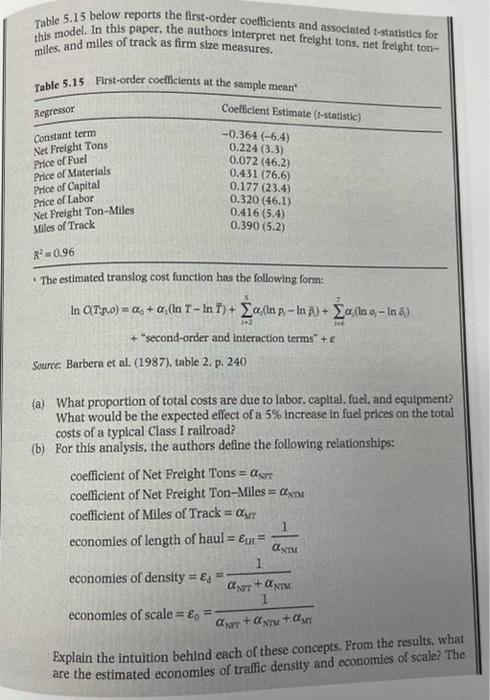
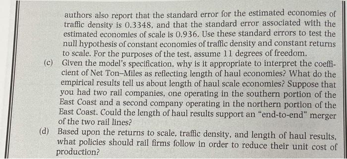
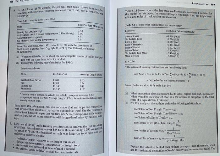
9. Barbera et al. (1987) used a translog cost function to analyze the cost structure for all Class I railroads (revenues over $253.7 million annually, 1993 dollars) fe the period 197983. The dependent variable was long-run total costs and the explanatory variables included: the level of output, measured as net freight ton-miles the operating characteristic, measured as net freight tons the network size, measured as miles of track operated the prices of inputs for labor, capital, fuel, and materials . . Table 5.15 below reports the first-order coefficients and associated t-statistics for this model. In this paper, the authors interpret net freight tons, net freight ton- miles, and miles of track as firm size measures. Table 5.15 First-order coefficients at the sample mean Regressor Constant term Net Freight Tons Price of Fuel Price of Materials Price of Capital Price of Labor Net Freight Ton-Miles Miles of Track Coelficient Estimate (t-statistic) -0.364 (-6.4) 0.224 (3.3) 0.072 (46.2) 0.431 (76.6) 0.177 (23.4) 0.320 (46.1) 0.416 (5.4) 0.390 (5.2) R=0.96 The estimated translog cost function has the following form: In aT.p.) = a + a, (In T- In 1)+ a(Inp - In 1) + a(In o, - In 3) + "second-order and interaction terms + E Source: Barbera et al. (1987). table 2. p. 240 (a) What proportion of total costs are due to labor, capital, fuel, and equipment? What would be the expected effect of a 5% increase in fuel prices on the total costs of a typical Class I railroad? (b) For this analysis, the authors define the following relationships: coefficient of Net Freight Tons = axt coefficient of Net Freight Ton-Miles = x coefficient of Miles of Track = economies of length of haul = Eu= AXTM 1 economies of density = = UNIT 1 economies of scale = Ep = arm + a.ru have + ONTM Explain the intuition behind each of these concepts. From the results, what are the estimated economies of traffic density and economies of scale? The authors also report that the standard error for the estimated economies of traffic density is 0.3348, and that the standard error associated with the estimated economies of scale is 0.936. Use these standard errors to test the null hypothesis of constant economies of traffic density and constant returns to scale. For the purposes of the test, assume 11 degrees of freedom. (c) Given the model's specification, why is it appropriate to interpret the coeffi- cient of Net Ton-Miles as reflecting length of haul economies? What do the empirical results tell us about length of haul scale economies? Suppose that you had two rail companies, one operating in the southern portion of the East Coast and a second company operating in the northern portion of the East Coast. Could the length of haul results support an "end-to-end" merger of the two rail lines? (d) Based upon the returns to scale, traffic density, and length of haul results. what policies should rail firms follow in order to reduce their unit cost of production? 18 FO REGON 199 8. In 1958. Reler (1971) Identified the per seat-mile costs shown in table dated with four major Intercity modes of travel: rail. Bir automobil Table 5.15 below reports the flest-order coeficients and cated state for The model. In this paper, the authors interpret set freight tons, et freight tro- mies, and miles of track as firm ste mesures. Intery but Table 5.14 city medal.com 1965 Vale Cost Per Semi-Mile Table 5.15 Pins-onder coefficients at the momplement Ciech Inclus 200-metre Alle 1011, 256 coloration. 250-mile trip) Automobile woni) Ridecar trating 240 passengers 1.44 3.00 4.5 1.5 Regressor Castantem Not Freight Tons Pre of Fuel Price of Materials Price of Capital The oftar Net Freight Ton-Miles Miles of Track -0.364-6,41 0.2243 0.072666 0.431 (76,60 0.177 (23.4 0.120 (461) 0.416.4) D.10 (52) Sunt relied trom Keeler (1971) talle 7.p. 166). with the perminton of The intensity of Chicago Pres. Copyright 1971 by The Uttelty of Chicas Alights What does this table tell us about the cost competitiveness of railin compers Ison with the other three intercity modes? ibi Consider the following sets of statistics for 1990: Internal costa Mode Per Mile Cost Average length of the Certified Air Care 11.02 NO3 12.85 274 Inicy Blus 11.55 141 Auto 11.3 -0.96 The estimated translog con fonction has the following formi In a + (n T-In) Salons - 14 ). "condorder and interactions" Se Barbern et al. (1987). table 2. 240 wile colofopending a vehicle per vehicle occupantes 1.2 perhidea 1990. Average length of Trip for automobile is based y con trip Based upon this information, crn you conclude that rail trips are competit with a tripod How about interdity bus or automobile tripw? Use the concert de conomies of distance to argue that all trip will be more competitive with her haul dir tripe, but will be los compete with longer-haul intercity bus and up trips Burberal. (1957) und a translog cost function to analyze the cost structure for allus Trailroads revues over $253.7 million annually. 1993 dollar the period 1979-83. The dependent variable was long-run total cost and the (w) What proportion of total costs are due to labor, capital fuel and equipment What would be the expected effect of increase in fuel prices on the total costs of a typical Class I railroad? (b) For this analysis, the authors define the following relationship oefficient of Net Freight Toner coefficient of Net Preght To Me coefficient of Miles of Track 1 economies of length of haul 1 economies of density aux 1 economies of scale to axy Explain the intuition behind each of these concepts. From the results what are the estimated economies of trafic density and economies of scale? The plaatory rares included: the level of output. measured as net freight ton-miles . the opening characteristic measured as net freight tons the network stat, mesured as miles of track operated the prices of inputs for labor, capital, fuel, and materials 9. Barbera et al. (1987) used a translog cost function to analyze the cost structure for all Class I railroads (revenues over $253.7 million annually, 1993 dollars) fe the period 197983. The dependent variable was long-run total costs and the explanatory variables included: the level of output, measured as net freight ton-miles the operating characteristic, measured as net freight tons the network size, measured as miles of track operated the prices of inputs for labor, capital, fuel, and materials . . Table 5.15 below reports the first-order coefficients and associated t-statistics for this model. In this paper, the authors interpret net freight tons, net freight ton- miles, and miles of track as firm size measures. Table 5.15 First-order coefficients at the sample mean Regressor Constant term Net Freight Tons Price of Fuel Price of Materials Price of Capital Price of Labor Net Freight Ton-Miles Miles of Track Coelficient Estimate (t-statistic) -0.364 (-6.4) 0.224 (3.3) 0.072 (46.2) 0.431 (76.6) 0.177 (23.4) 0.320 (46.1) 0.416 (5.4) 0.390 (5.2) R=0.96 The estimated translog cost function has the following form: In aT.p.) = a + a, (In T- In 1)+ a(Inp - In 1) + a(In o, - In 3) + "second-order and interaction terms + E Source: Barbera et al. (1987). table 2. p. 240 (a) What proportion of total costs are due to labor, capital, fuel, and equipment? What would be the expected effect of a 5% increase in fuel prices on the total costs of a typical Class I railroad? (b) For this analysis, the authors define the following relationships: coefficient of Net Freight Tons = axt coefficient of Net Freight Ton-Miles = x coefficient of Miles of Track = economies of length of haul = Eu= AXTM 1 economies of density = = UNIT 1 economies of scale = Ep = arm + a.ru have + ONTM Explain the intuition behind each of these concepts. From the results, what are the estimated economies of traffic density and economies of scale? The authors also report that the standard error for the estimated economies of traffic density is 0.3348, and that the standard error associated with the estimated economies of scale is 0.936. Use these standard errors to test the null hypothesis of constant economies of traffic density and constant returns to scale. For the purposes of the test, assume 11 degrees of freedom. (c) Given the model's specification, why is it appropriate to interpret the coeffi- cient of Net Ton-Miles as reflecting length of haul economies? What do the empirical results tell us about length of haul scale economies? Suppose that you had two rail companies, one operating in the southern portion of the East Coast and a second company operating in the northern portion of the East Coast. Could the length of haul results support an "end-to-end" merger of the two rail lines? (d) Based upon the returns to scale, traffic density, and length of haul results. what policies should rail firms follow in order to reduce their unit cost of production? 18 FO REGON 199 8. In 1958. Reler (1971) Identified the per seat-mile costs shown in table dated with four major Intercity modes of travel: rail. Bir automobil Table 5.15 below reports the flest-order coeficients and cated state for The model. In this paper, the authors interpret set freight tons, et freight tro- mies, and miles of track as firm ste mesures. Intery but Table 5.14 city medal.com 1965 Vale Cost Per Semi-Mile Table 5.15 Pins-onder coefficients at the momplement Ciech Inclus 200-metre Alle 1011, 256 coloration. 250-mile trip) Automobile woni) Ridecar trating 240 passengers 1.44 3.00 4.5 1.5 Regressor Castantem Not Freight Tons Pre of Fuel Price of Materials Price of Capital The oftar Net Freight Ton-Miles Miles of Track -0.364-6,41 0.2243 0.072666 0.431 (76,60 0.177 (23.4 0.120 (461) 0.416.4) D.10 (52) Sunt relied trom Keeler (1971) talle 7.p. 166). with the perminton of The intensity of Chicago Pres. Copyright 1971 by The Uttelty of Chicas Alights What does this table tell us about the cost competitiveness of railin compers Ison with the other three intercity modes? ibi Consider the following sets of statistics for 1990: Internal costa Mode Per Mile Cost Average length of the Certified Air Care 11.02 NO3 12.85 274 Inicy Blus 11.55 141 Auto 11.3 -0.96 The estimated translog con fonction has the following formi In a + (n T-In) Salons - 14 ). "condorder and interactions" Se Barbern et al. (1987). table 2. 240 wile colofopending a vehicle per vehicle occupantes 1.2 perhidea 1990. Average length of Trip for automobile is based y con trip Based upon this information, crn you conclude that rail trips are competit with a tripod How about interdity bus or automobile tripw? Use the concert de conomies of distance to argue that all trip will be more competitive with her haul dir tripe, but will be los compete with longer-haul intercity bus and up trips Burberal. (1957) und a translog cost function to analyze the cost structure for allus Trailroads revues over $253.7 million annually. 1993 dollar the period 1979-83. The dependent variable was long-run total cost and the (w) What proportion of total costs are due to labor, capital fuel and equipment What would be the expected effect of increase in fuel prices on the total costs of a typical Class I railroad? (b) For this analysis, the authors define the following relationship oefficient of Net Freight Toner coefficient of Net Preght To Me coefficient of Miles of Track 1 economies of length of haul 1 economies of density aux 1 economies of scale to axy Explain the intuition behind each of these concepts. From the results what are the estimated economies of trafic density and economies of scale? The plaatory rares included: the level of output. measured as net freight ton-miles . the opening characteristic measured as net freight tons the network stat, mesured as miles of track operated the prices of inputs for labor, capital, fuel, and materials