Question One Only please

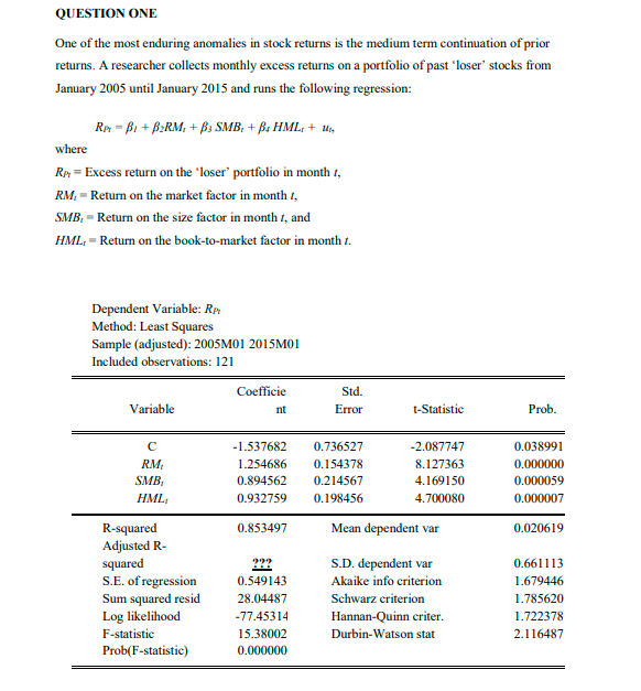
QUESTION ONE CONTINUED a) Briefly explain the purpose of the above regression. (6 Marks) b) Comment on the sign and significance of the estimated coefficients. (6 Marks) c) Obtain a 95% confidence interval for B2 and a 90% confidence interval for B3. Briefly comment on your results. (7 Marks) Compute the adjusted Rof the above regression. (6 Marks) TOTAL 25 MARKSI END OF QUESTION ONE QUESTION TWO a) Define the term autocorrelation'. Explain why there might often be autocorrelation in the errors of models using financial time series data. (7 Marks) b) Describe the consequences of autocorrelation for the properties of the OLS estimators and for statistical inference. (6 Marks) Outline the 'Breusch-Godfrey' test for autocorrelation and explain when it will be preferred to the Durbin-Watson test. (6 Marks) Assuming autocorrelation is present, critically describe any possible solutions. (6 Marks) c) QUESTION ONE One of the most enduring anomalies in stock returns is the medium term continuation of prior returns. A researcher collects monthly excess returns on a portfolio of past 'loser' stocks from January 2005 until January 2015 and runs the following regression: RA =B1 + BRM+BSMB+B. HML: + Wig where Rp = Excess return on the 'loser" portfolio in month I, RM = Return on the market factor in month t, SMB = Return on the size factor in month t, and HML, = Return on the book-to-market factor in month t. Dependent Variable: R Method: Least Squares Sample (adjusted): 2005M01 2015M01 Included observations: 121 Coefficie nt Std. Error Variable t-Statistic Prob. RM SMB HML -1.537682 1.254686 0.894562 0.932759 0.736527 0.154378 0.214567 0.198456 -2.087747 8.127363 4.169150 4.700080 0.038991 0.000000 0.000059 0.000007 0.853497 Mean dependent var 0.020619 R-squared Adjusted R- squared S.E. of regression Sum squared resid Log likelihood F-statistic Prob(F-statistic) 0.549143 28.04487 -77.45314 15.38002 0.000000 S.D. dependent var Akaike info criterion Schwarz criterion Hannan-Quinn criter. Durbin-Watson stat 0.661113 1.679446 1.785620 1.722378 2.116487 QUESTION ONE CONTINUED a) Briefly explain the purpose of the above regression. (6 Marks) b) Comment on the sign and significance of the estimated coefficients. (6 Marks) c) Obtain a 95% confidence interval for B2 and a 90% confidence interval for B3. Briefly comment on your results. (7 Marks) Compute the adjusted Rof the above regression. (6 Marks) TOTAL 25 MARKSI END OF QUESTION ONE QUESTION TWO a) Define the term autocorrelation'. Explain why there might often be autocorrelation in the errors of models using financial time series data. (7 Marks) b) Describe the consequences of autocorrelation for the properties of the OLS estimators and for statistical inference. (6 Marks) Outline the 'Breusch-Godfrey' test for autocorrelation and explain when it will be preferred to the Durbin-Watson test. (6 Marks) Assuming autocorrelation is present, critically describe any possible solutions. (6 Marks) c) QUESTION ONE One of the most enduring anomalies in stock returns is the medium term continuation of prior returns. A researcher collects monthly excess returns on a portfolio of past 'loser' stocks from January 2005 until January 2015 and runs the following regression: RA =B1 + BRM+BSMB+B. HML: + Wig where Rp = Excess return on the 'loser" portfolio in month I, RM = Return on the market factor in month t, SMB = Return on the size factor in month t, and HML, = Return on the book-to-market factor in month t. Dependent Variable: R Method: Least Squares Sample (adjusted): 2005M01 2015M01 Included observations: 121 Coefficie nt Std. Error Variable t-Statistic Prob. RM SMB HML -1.537682 1.254686 0.894562 0.932759 0.736527 0.154378 0.214567 0.198456 -2.087747 8.127363 4.169150 4.700080 0.038991 0.000000 0.000059 0.000007 0.853497 Mean dependent var 0.020619 R-squared Adjusted R- squared S.E. of regression Sum squared resid Log likelihood F-statistic Prob(F-statistic) 0.549143 28.04487 -77.45314 15.38002 0.000000 S.D. dependent var Akaike info criterion Schwarz criterion Hannan-Quinn criter. Durbin-Watson stat 0.661113 1.679446 1.785620 1.722378 2.116487