Question:

Show that it is undecidable, given the source code of a program Q, to tell whether or not any of the following is true:

(i) Q halts on input 0.

(ii) Q is total - that is, Q(y) halts for all y.

(iii) Q(y) = true for all y.

(iv) The set of y on which Q halts is nite.

(v) There is a y such that Q(y) = y.

(vi) Given a second program R, Q is equivalent to R. That is, even though Q and R have different source codes, they compute the same partial function - for all y, either Q(y) and R(y) both halt and return the same answer, or neither halts.

Prove each of these by reducing Halting to them. That is, show to how convert an instance (P, x) of Halting to an instance of the problem above. For instance, you can modify P's source code, or design a new program that calls P as a subroutine. Each of these is asking for a Turing reduction; your reduction does not necessarily have to map yes-instances to yes-instances and no-instances to no-instances - all that matters is that if you could solve the problem, then you could solve Halting.

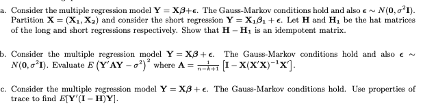
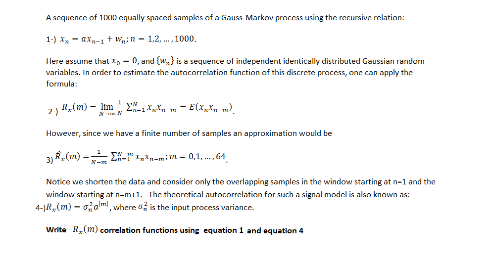
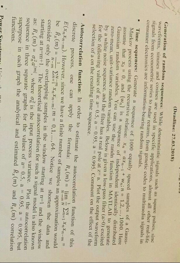
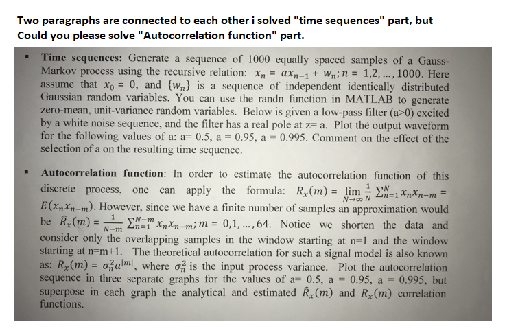
a. Consider the multiple regression model Y = XA+e. The Gauss-Markov conditions hold and also e ~ N(0, o' 1). Partition X = (X1, X2) and consider the short regression Y = X1/1 + 6. Let H and H, be the hat matrices of the long and short regressions respectively. Show that H - He is an idempotent matrix. b. Consider the multiple regression model Y = XA + e. The Gauss-Markov conditions hold and also e N(0, o'I). Evaluate E (Y'AY - o') where A = I-X(X'X) 'X']. c. Consider the multiple regression model Y = X8 + e. The Gauss-Markov conditions hold. Use properties of trace to find E[Y'(I - H)Y].A sequence of 1000 equally spaced samples of a Gauss-Markov process using the recursive relation: 1-) Xn = axn-1+ Win = 1,2, ...,1000. Here assume that Xo = 0, and {W, ) is a sequence of independent identically distributed Gaussian random variables. In order to estimate the autocorrelation function of this discrete process, one can apply the formula: N-co N 2-) Rx(m) = lim = En=1XXn-m = E(Xn*n-m). However, since we have a finite number of samples an approximation would be 3) Rx(m) =- N-m 2n=1 XinXin-mim = 0,1, ..., 64 Notice we shorten the data and consider only the overlapping samples in the window starting at n=1 and the window starting at n=m+1. The theoretical autocorrelation for such a signal model is also known as: 4-)Rx(m) = on all, where On is the input process variance. Write Rx(m) correlation functions using equation 1 and equation 4(Deadline: 27.03.2018) Generation of random sequences: While deterministic signals such as square pulses, sinc waveforms, sinuses and cosines are used in specific applications, almost all other real-life signals from econometric series to radar returns, from genetic codes to multimedia signals in consumer electronics are information-bearing random signals. Time sequences: Generate a sequence of 1000 equally spaced samples of a Gauss- Markov process using the recursive relation: X = ax,_ + win = 1,2, ..., 1000. Here assume that Xo = 0. and {Wn} is a sequence of independent identically distributed Gaussian random variables. You can use the randn function in MATLAB to generate zero-mean. unit-variance random variables. Below is given a low-pass filter (a>0) excited by a white noise sequence, and the filter has a real pole at z- a. Plot the output waveform for the following values of a: a=0.5, a = 0.95, a = 0.995. Comment on the effect of the selection of a on the resulting time sequence. Autocorrelation function: In order to estimate the autocorrelation function of this discrete process, one can apply the formula: R. (m) = lim - EN_ N-CON Ln=1XnXn-m= E(Xn*n-m). However, since we have a finite number of samples an approximation would be Rx(m) = N_m Zn=1 XnXn-mim = 0,1, ...,64. Notice we shorten the data and consider only the overlapping samples in the window starting at n=1 and the window starting at n-m+1. The theoretical autocorrelation for such a signal model is also known as: R(m) = ozalm. where on is the input process variance. Plot the autocorrelation sequence in three separate graphs for the values of a= 0.5, a = 0.95, a = 0.995, but superpose in each graph the analytical and estimated Rx (m) and R. (m) correlation functions.Two paragraphs are connected to each other i solved "time sequences" part, but Could you please solve "Autocorrelation function" part. Time sequences: Generate a sequence of 1000 equally spaced samples of a Gauss- Markov process using the recursive relation: An = axn-1 + Wn; n = 1,2,..., 1000. Here assume that Xo = 0, and {w,} is a sequence of independent identically distributed Gaussian random variables. You can use the randn function in MATLAB to generate zero-mean, unit-variance random variables. Below is given a low-pass filter (a>0) excited by a white noise sequence, and the filter has a real pole at z= a. Plot the output waveform for the following values of a: a= 0.5, a = 0.95, a = 0.995. Comment on the effect of the selection of a on the resulting time sequence. Autocorrelation function: In order to estimate the autocorrelation function of this discrete process, one can apply the formula: Rx(m) = lim = > N-co N 2n=1*n*n-m = E(XXn-m). However, since we have a finite number of samples an approximation would be Rx(m) = -EN minxn-mim = 0,1,...,64. Notice we shorten the data and consider only the overlapping samples in the window starting at n=1 and the window starting at n=m+1. The theoretical autocorrelation for such a signal model is also known as: Rx(m) = opalml, where o? is the input process variance. Plot the autocorrelation sequence in three separate graphs for the values of a= 0.5, a = 0.95, a = 0.995, but superpose in each graph the analytical and estimated Rx(m) and Rx(m) correlation functions