Questions 1 and 2, please show work in excel.

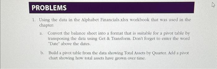
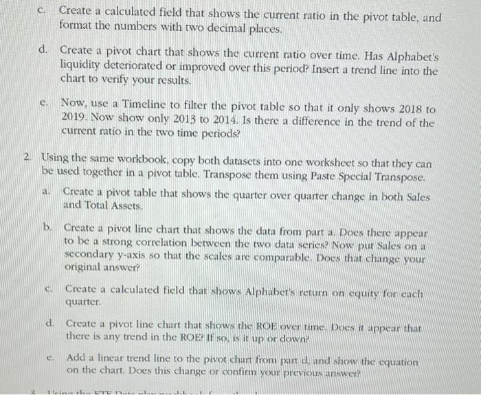
1. Using the data in the Alphabet Financials xlsx workbook that was used in the chapter: a. Convert the balance sheet into a format that is suitable for a pivot table by transposing the data using Get \& Transform. Don't forget to enter the word "Date" above the dates. b. Build a pivot table from the data showing Total Assets by Quarter. Add a pivot chart showing how total assets have grown over time. c. Create a calculated field that shows the current ratio in the pivot table, and format the numbers with two decimal places. d. Create a pivot chart that shows the current ratio over time. Has Alphabet's liquidity deteriorated or improved over this period? Insert a trend line into the chart to verify your results. e. Now, use a Timeline to filter the pivot table so that it only shows 2018 to 2019. Now show only 2013 to 2014. Is there a difference in the trend of the current ratio in the two time periods? 2. Using the same workbook, copy both datasets into one worksheet so that they can be used together in a pivot table. Transpose them using Paste Special Transpose. a. Create a pivot table that shows the quarter over quarter change in both Sales and Total Assets. b. Create a pivot line chart that shows the data from part a. Does there appear to be a strong correlation between the two data series? Now put Sales on a secondary y-axis so that the scales are comparable. Does that change your original answer? c. Create a calculated field that shows Alphaber's return on equity for ench quarter. d. Create a pivot line chart that shows the ROE over rime. Docs it appear that there is any trend in the ROE? If so. is it up or down? e. Add a linear trend line to the pivot chart from part d, and show the equation on the chart. Does this change or confirm your previous answer? 1. Using the data in the Alphabet Financials xlsx workbook that was used in the chapter: a. Convert the balance sheet into a format that is suitable for a pivot table by transposing the data using Get \& Transform. Don't forget to enter the word "Date" above the dates. b. Build a pivot table from the data showing Total Assets by Quarter. Add a pivot chart showing how total assets have grown over time. c. Create a calculated field that shows the current ratio in the pivot table, and format the numbers with two decimal places. d. Create a pivot chart that shows the current ratio over time. Has Alphabet's liquidity deteriorated or improved over this period? Insert a trend line into the chart to verify your results. e. Now, use a Timeline to filter the pivot table so that it only shows 2018 to 2019. Now show only 2013 to 2014. Is there a difference in the trend of the current ratio in the two time periods? 2. Using the same workbook, copy both datasets into one worksheet so that they can be used together in a pivot table. Transpose them using Paste Special Transpose. a. Create a pivot table that shows the quarter over quarter change in both Sales and Total Assets. b. Create a pivot line chart that shows the data from part a. Does there appear to be a strong correlation between the two data series? Now put Sales on a secondary y-axis so that the scales are comparable. Does that change your original answer? c. Create a calculated field that shows Alphaber's return on equity for ench quarter. d. Create a pivot line chart that shows the ROE over rime. Docs it appear that there is any trend in the ROE? If so. is it up or down? e. Add a linear trend line to the pivot chart from part d, and show the equation on the chart. Does this change or confirm your previous